TECHNICAL GALFIT FAQ
How do I determine the initial parameters?
By all means: just take a guess and see what happens.
One may think that taking a guess is unwise, perhaps having a prior notion
about parameter degeneracy, local minimum solutions, or other things
regarding Levenberg-Marquardt algorithms. They are definitely legitimate
concerns, and there's definitely a limit as to how far initial guesses can
be off otherwise guesses wouldn't be necessary. However, it is much more
common for people to think that problems are all due to parameter degeneracy
or local minimum solutions rather than due to other, more responsible and
less obvious, causes. For example, neighboring contamination, incorrect
sigma images, sky level determined independently and held fixed to incorrect
local value, flatfield non-uniformity, image fitting size, a subtle bug in
one's code, etc., all can lead to incorrect and unexpected outcomes.
Blaming the wrong cause, it is unlikely any algorithm, downhill gradient or
otherwise, would be able to find the correct solution because the desired
solution would not yield the best numerical merit, e.g. χ2.
There are ways to figure out the true causes, and knowing how to make
accurate diagnosis is of course important for both getting the correct
answer and for not performing ill-conceived follow-up analysis to ostensibly
"correct the errors," which can further lead to other problems or, worse, a
false sense of security. For example, if the sigma image is wrong and one
ascribes systematic errors to parameter degeneracy, it may lead one to try
and correct the errors in the final fit parameters, leading to solutions
that are far worse than correcting the problem at the source (as seen here).
In practice, even for an algorithm like Levenberg-Marquardt, which is a
down-hill gradient type algorithm, concerns about how good the initial
parameters need to be are often a bit overstated for galaxy fitting.
Whereas people worry themselves over finding initial guesses that are more
accurate than 30-50%, which is nice, the actual allowed tolerances are often
far larger: on the order of many hundred, thousand, sometimes even tens or
hundreds of thousand, percent, depending on the signal-to-noise and the
complexity of the model. Suffice to say that, for single component
Sérsic fits, if your guesses are off by less than 100%, they're
probably fine. This is not always the case for multi-component fits of a
single galaxy. The more number of components one uses, the better and
faster the algorithm will converge on a solution if the guesses are more
accurate.
This discussion is not meant to persuade anyone that numerical degeneracies
or local minima don't exist. Rather, with enough experience, the initial
concerns usually give way to a more accurate understanding and hopefully
better application of the software tool. There is no shortcut to learning
about the true versus imagined or preconceived limitations of the analysis
technique except by trying, especially because galaxy profiles are complex
things. However, there are some recipes, rules of thumb, gained through
experience:
- Be daring and open to just
trying. Develop an intuition by taking guesses: If there's nothing
strange or wrong with the data image itself, and the (conversion to get)
sigma image is correct, and all bad pixel regions (zero values, bad columns,
gaps, cosmic rays, saturated stars, etc., etc.) are masked out, and
neighboring objects are dealt with (masked out or fitted simultaneously),
then most of the time a reasonably crude (see next item) guess should be
fine, and the fit should converge on a sensible answer, pretty much
regardless of what numbers you start from. GALFIT is not that finicky.
However, if it does behave in finicky ways, usually the problem can be
traced to something in the data or the sigma image, or perhaps the priors
about the models are not appropriate.
- What does "reasonably crude" mean?:
It's useful to have numbers to "hang a hat on," so-to-speak. So let's just
say for a single component fit,
using the Sérsic profile ,
reasonably crude is something like: brightness to within about 3, 4,
occasionally even 5 magnitudes (factors of 15, 40, 100); size to within a
factor of 30; axis ratio to within 0.5; position angle to within 60 degrees;
Sérsic index to within 2-ish. There are actually no hard and fast
rules because factors such as noise, neighboring objects, unanticipated
issues with the data, etc., can narrow or widen the tolerances. But the
point is that one should focus more on what the fits mean either due to
other things in the image, or physically when using different models, rather
than about getting the initial parameters. The one caveat is when all
the parameters are off by extreme values simultaneously, then GALFIT
may crash immediately, or may iterate to the end without changing any of the
parameters by much. There are some profile functions which are more
sensitive to initial guesses than others, e.g. the Nuker, so one has to
develop an intuition individually for those.
- What if I want to fit more than one component
to an object? When fitting two or more components to a single
object (as opposed to multiple objects at once), one has to be more careful.
In this situation, it is usually better to start by fitting a single
component. Then, take the best fit result and add on top of that, allowing
both components to adjust. This is done by adding another component to the
"galfit.NN" file (NN is an integer) which stores the most recent best
fitting parameters. For more components, repeat the process. The reason
for a step-wise approach is to guarantee that the initial parameters are not
wildly off for two or more components simultaneously, which is worse
than having initial guesses be badly off for a single component: when
components overlap, bad initial guesses compound. Another reason is that
sometimes your eyes may mislead, that what you think may be the second
strongest component may not actually be, and it is better to let GALFIT
determine what it sees as reasonable by starting from the ground up.
- Magnitude is the most common error people
make in initial guesses: When making initial guesses, the
magnitude parameter is the one people have some difficulty guessing
well. Or, perhaps an user may not be unaware that he/she is analyzing
an image with a missing or improper exposure time keyword or value.
For instance, when an image is normalized by the exposure time, i.e.
ADUs in counts/second, often the header keyword continues to report
the total exposure time rather than one second. That is bad practice
because it is then not obvious what the magnitude zeropoint refers to.
So if the exposure time says 100 seconds or 1000 seconds, the initial
guess for the magnitude would be off by 5 or 7.5, magnitudes,
respectively, or more. A quick-and-dirty way to make sure the
magnitude is ok is simply to do a quick computation:
mag = -2.5 log10 [(total flux in a box - rough sky value × number
of pixel in that box) / EXPTIME] + magzpt.
One can do this via simple aperture photometry. This calculation
doesn't have to be accurate and the region doesn't have to be very
large (but it can be if one likes). Even the crudest estimate is
usually good to much better than 1 mag, i.e. a factor of 2.5.
- Help! GALFIT keeps going crazy even though
the initial parameters are reasonable and the data/sigma images are fine.
Why?: There could be several reasons. Sometimes it may be that one
is trying to fit a single component model to a region that requires several
components. For instance, if there's a fairly bright nuclear point source
near or sitting on top of a galaxy, and one is fitting a single component,
that may deserve more attention than the galaxy, and masking out the
neighbor may not be enough. Or, the sky flatfielding may be bad. Or, the
sky may be ill determined in the image because the fitting region is too
small. What to do about these situations would depend on the science goal.
Feel free to contact me for support at email address located bottom of the
page if it is not clear what to do. I will likely ask to see your data
(either in FITS file or, e.g. in JPG) and analysis, or ask about the purpose
of the analysis if the solution is dependent on the science-goal.
- If none of the suggestions help,
before giving up, please read the Top 10 Rules of
Thumb for galaxy fitting.
Why is the GALFIT output image blank?
The output image produced by GALFIT is an image block, with the
zeroth image slice being blank. Thus displaying the image without
specifying the proper image slice will result in a blank image being
displayed. To see the image block using DS9, go to "File"==>"Open
Other"==>"Open Multi-Ext as Data Cube." To display it using IRAF,
type "display imgblock[1]". Use [2] and [3] to see other image
slices. There are several ways to show image blocks in IDL and other
software as well.
How biased are the size and luminosity measurements
by low signal-to-noise when you can't see outer regions of galaxies?
A question people often have is whether signal-to-noise (S/N) can cause
systematic biases in the fitting parameters. Some believe model fitting is
likely to underestimate the size and luminosity parameters because our
intuitions tells us that we can see only the "the tip of the iceberg," thus
the code is likely to miss out on flux that is beneath the noise. It is
also common to think that one has to account for all the structural
components in galaxies in order to properly measure the total luminosity and
the global size. Therefore, if the outer wings have too low S/N, we can't
account for them, so the measurements are likely to be biased toward smaller
values. This belief often leads one to choose non-parametric techniques,
like aperture or curve-of-growth (COG,
see
below) analyses, because they do not rely on one's knowledge about
galaxy structures to measure the luminosity and sizes. This section and
the one below explain why adopting
non-parametric techniques actually may steer one closer to pitfalls which
one is consciously trying to avoid.
The reason why parametric techniques are very useful, and often better
than non-parametric techniques, in low S/N situations is that parametric
fitting is fundamentally about model testing. Model testing is a
strength, not a weakness, because it can use both the signal and the noise
information via a sigma image, combined together
in χ2, in a rigorous and, just
as importantly, proper, manner. In other words, in low S/N
situations when we just see the "tip of the iceberg" of galaxy centers
model testing tries to figure out how much extended wing is allowed by the
noise. Noise is information, and an important one at that. If
the noise is large, it doesn't mean that the model "doesn't see" the
galaxy. Quite the opposite, it means that more and more extended models
are consistent with the noise, which is why the errorbar on size
becomes larger and larger. Indeed, it is incorrect to think that because
we only see the tip, that must also be what a parametric algorithm "sees,"
and expect the code to behave according to our intuition. Another factor
contributing to a misconception is a belief that parametric analysis is
highly sensitive to parameter degeneracy -- that critique is analyzed here and shown not to be well deserved in
general. Lastly, it is common to think that parametric analysis needs to
account for all the components for it to work properly. If one is
interested in the physical meaning of the multiple components of a galaxy
then that is true but it's for the interpretation to be clear, not
because otherwise the fit is somehow wrong in some abstract sense.
However, for single component fits the meaning is clear: it is about
finding a global model that minimizes the residuals. And that does not
necessitate the profile function to be perfect for the technique to work
properly. It would certainly be better for the profile functions to be
more accurate through multi-component fitting to further reduce the
residuals. This is possible to do in an automated way if one does not
need to know about the meaning of the subcomponents, but rather to only
need to measure the total flux and size.
To illustrate the above claims it is useful to turn to some simple
simulations. Figures 1a, 1b, and
1c, show 3 controlled experiments based on simulated
galaxies, each one created to have a bulge and a disk of 1:1 ratio in
luminosity (left panels), with parameters of the Sérsic profiles
shown in the top two rows. When analyzing the data, we fit a
single component Sérsic function (middle panels) to
purposefully simulate a model mismatch that is often a cited to be a main
source of weakness about the technique (see residuals in the top right
images). The simulation is repeated for several very high and very low
S/N situations. In a single component fit, one sees that the size
parameter for a single component is roughly half of the bulge and disk
sizes. This makes sense because the bulge-to-disk luminosity ratio is
created to be exactly 1-to-1.
SIMULATIONS OF GALAXY SIZE
MEASUREMENTS UNDER LOW AND HIGH SIGNAL-TO-NOISE REGIMES
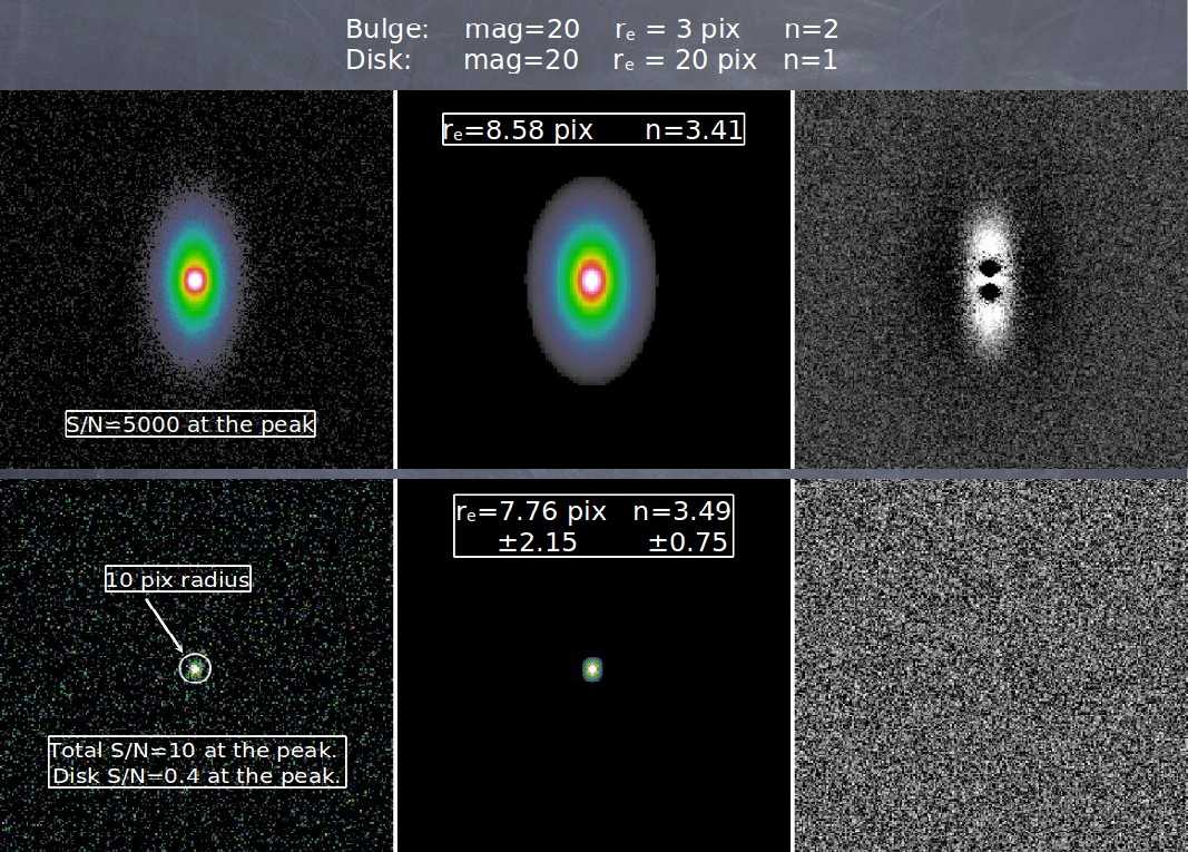
Figure 1a: a two component model
with intrinsic parameters shown on the top row, outside the images.
Top row: the first image (left) shows a model with very high
S/N of 5000 at the peak, the middle image shows a single component fit
to the data, finding the parameters shown in square box, and the third
image (right) shows the residuals from the fit.
Bottom Row:
images showing a similar sequence for the same galaxy now with very
low S/N of only 10 at the peak. Despite the fact that the galaxies
have very different S/N levels, despite the fact that a single
component model is a bad fit to the data, and despite the fact that
the disk component has been completely faded below the noise in the
second simulation, the size and concentration parameters are measured
to be nearly identical to within the error bars given by GALFIT.
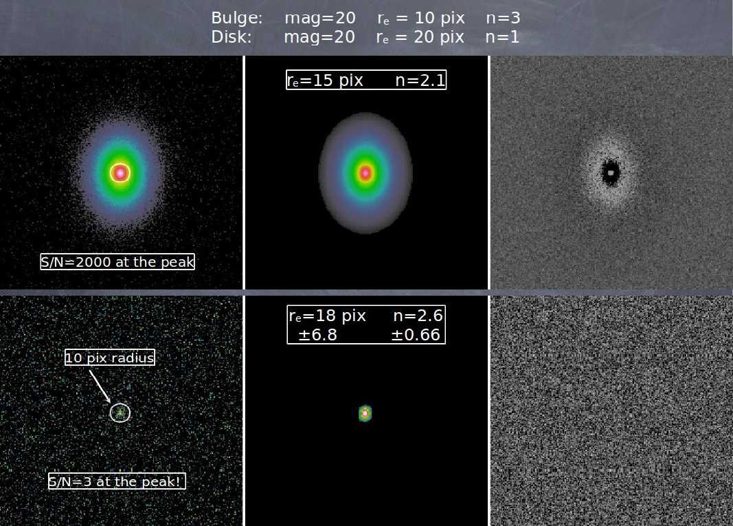
Figure 1b: See Figure 1a for
details. Similar simulation as Figure 1a except with different bulge
size and concentration index. Again, the sizes measured are
essentially identical between low and high S/N simulations to within
the errors, despite vast differences in S/N.
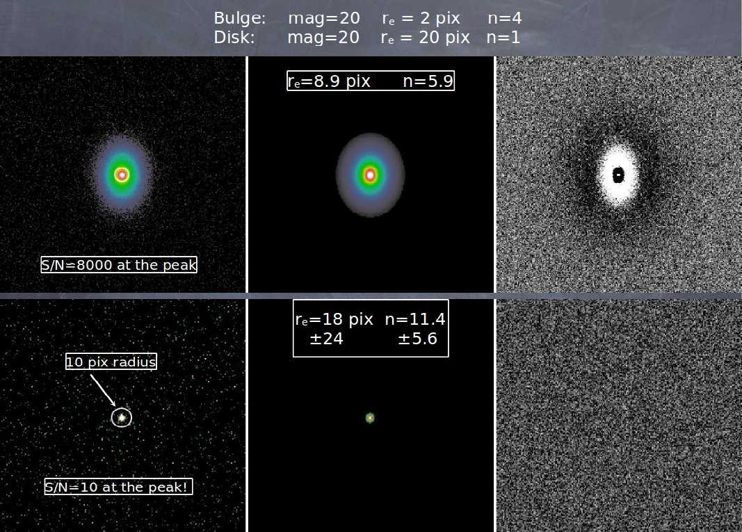
Figure 1c: See Figure 1a for
details. Similar simulation as Figure 1a except with different bulge
size and concentration index. Here, although the size estimate of the
fainter image is larger than for the high S/N image, it is still
within the errorbar. Moreover, the direction is toward finding a
larger size for the fainter image, contrary to expectations
that fading of the outer regions causes the size estimate to be biased
toward a lower value.
As we can see from the above simulations, the notion that model mismatch
and S/N would preferentially bias parametric analysis toward finding
smaller sizes and lower luminosity is not realized in practice. When
statistics are properly taken into account in low S/N simulations, the
noisier data are consistent with a wider range of acceptable models, which
produces parameters that have larger errorbars than high S/N simulations.
But the central values are nevertheless consistent between very high and
extremely low S/N situations to within the errorbar. In contrast, the
discussion immediately below explains why
non-parametric analyses,
which often do not properly account for noise in the data, may cause one
to underestimate galaxy sizes and luminosities.
Why determine galaxy sizes and luminosities with
parametric instead of non-parametric techniques?
Measuring galaxy sizes and luminosities is a tricky business because most
galaxies don't have sharp edges. There are two general approaches to
measuring sizes and luminosities: non-parametric and parametric.
Non-parametric techniques involve aperture photometry of some sort like
curve-of-growth (COG) analysis, whereas parametric techniques involve
fitting functions to images of galaxies. The most common definitions of
"size" involve measuring flux inside a certain radius, such as the
half-light-radius, or perhaps some kind of scalelength parameter in the
case of functional model fitting. Luminosities are often measured using
aperture flux inside a certain radius, or flux integrated out to some
surface brightness level, or based on the total flux from analytic models
or COG. Both parametric and non-parametric techniques have benefits and
drawbacks, some of which are discussed in this section.
The above section explains why parametric
techniques are useful in low S/N situations because of the premise of
model testing.
In contrast, non-parametric techniques, like the curve-of-growth (COG)
analysis, are not about hypothesis testing. They often use the noise
information to decide where to stop extracting a galaxy profile. As such,
the technique indeed corresponds more to the notion of "what you see is what
you get" because the noisier the data, the closer in to the center the
galaxy seems to "end." COG and other non-parametric techniques often do in
fact use the noise information, but they often don't use it
properly. To be concrete, imagine trying to image a big, bright,
galaxy, say M31, with a very short exposure time, say a microsecond. The
galaxy is there in the image, but at such a low level that the image is
dominated by sky and readnoise. A curve-of-growth analysis usually compares
the flux gradient in an image to the noise in order to determine where the
galaxy "ends." It would therefore find a sky and readnoise dominated image
to be nearly perfectly flat, to very high precision when the image is large.
This would lead one to conclude with high confidence that the size of the
galaxy is 0 arcseconds in size, based on careful statistical analysis of the
background noise. This of course is the wrong answer. A parametric
analysis would tell you that the size is consistent with some central value,
but that value has uncertainty of ± ∞, which is another way to
say a model of 0 size is as good as one which is extremely large that
potentially includes the correct answer. Being highly uncertain about an
answer because of statistics is not wrong. However, being absolutely
certain about an incorrect answer is wrong, and that is a potential pitfall
with non-parametric analysis.
The relative benefits and drawbacks of parametric vs. non-parametric
techniques are summarized below:
-
Curve-of-Growth (COG) Analysis
(non-parametric): The COG technique uses apertures of growing
radii to sum up the light from a galaxy. Then one performs an analysis
on a curve of flux vs. aperture radius. As the aperture grows so does
the flux (sky subtracted) until that point when nearly all the light
is included and the COG approaches an asymptotic value. The
asymptotic flux value is taken to be total light from that galaxy, and
the size is then defined to be that radius which encloses some
fraction, often 50% or 90%, of the total light, or out to a certain
surface brightness.
Strengths:
- Model independent (sort of). This method does not
depend on the shape of the galaxy and is thus said to be model
independent. It can be applied to irregular galaxies and
regular galaxies, and galaxies of all profile types
(exponential, de Vaucouleurs, etc.). However, in practice this
is only partly true because one replaces parametric models with
interpretations about the behavior of the COG, or a
functional fit to COG to derive the asymptotic
integrated flux. Both of these processes are dependent on
assumptions (i.e. model) about the morphology and environment.
So while the notion is that the technique is robust for
galaxies across all shapes, in practice the
implementation may make the technique susceptible to
implicit model assumptions about the COG, as elaborated further
below concerning the weaknesses of this technique.
- Simplicity. It is easy to apply this technique across
galaxies of different shapes and sizes without making special
considerations.
Weaknesses:
- Does not account for the PSF. So when the galaxy size
is only a few times the size of the PSF FWHM or the resolution
element of the detector, or when the galaxy profile is steeply
concentrated, this technique is not very reliable for measuring
the size.
- Signal-to-noise (S/N), thus morphology, dependent. COG
and aperture techniques are to some degree S/N dependent as they
rely on being able to measure a gradient in galaxies. One can
only detect shallow profile gradients under very high S/N
situations. This would bias against measuring correct sizes for
galaxies that have slowly declining light profiles, such as
early-type or low surface brightness (relative to the noise)
galaxies. Another reason why this analysis is S/N dependent is
that, in the most common way of creating a COG, one has to first
subtract out the background sky: if the gradient is shallow with
low S/N, then the sky will be over-estimated, which then affects
the COG analysis. The decoupled, stepwise, approach makes it
always more likely to overestimate the sky, underestimate the
luminosity, and underestimate the size. See figure below for a concrete example.
- Crowding limited. COG does not work well if the
background is not flat, because the COG may not flatten out. And
the background may not be flat for all sorts of reasons, e.g.
crowded environments, overlapping galaxies, flatfielding errors,
bad sky subtraction, etc.. This gives rise to frequent dilemma:
if the COG starts to grow again at larger radii after showing
signs of flattening off, how does one decide what of the various
factors it is due to? How does one quantify? Making this
decision is non-trivial and intuition dependent. Without being
able to quantify how much those different variables matter,
decisions about this issue in turn impact the extraction of the
morphology parameters, making COG dependent on situation and
morphology.
-
Parametric fitting: The size
and luminosity parameters are built into the functional form of the
light profile model.
Strengths:
- Accounts for the PSF. The technique tests for
consistency of a galaxy profile with model functions by fitting
them to the data after convolving with the PSF. It is thus capable
of measuring or constraining the shape of the galaxy profile all
the way into the center. This is necessary if one needs to
measure galaxy sizes that are close to the PSF or pixel resolution
limit.
- Deals better with low S/N situations. It is often said
that analytic profiles can "extrapolate below the noise" to better
recover the total flux; this is an intuitive, generally correct,
although somewhat imprecise explanation. A more accurate way to
think about this is that in parametric analysis it is not just the
flux that matters, but the amount of flux compared to the expected
noise given that flux, encoded in the definition of
χ2. Because of χ2, weak signal
accumulates over large areas even when our eyes may not detect any
flux. These two facts mean that even if a galaxy has extended
wings that get washed out by the noise, a model with a large
envelope would still be consistent with the data given the noise
(sigma). In low S/N, the size and luminosity determinations are
more uncertain because models with smaller and larger sizes
may also be consistent with the noise. However, this does not
necessary mean the fit is biased one way or another. For biases
to appear the flux signal would have to be unrepresentative of the
sigma for that flux level. In contrast, in COG analysis the size
determination is based on measuring the gradient of the light
profile. Because the gradient does depend on the S/N, when there
is noise, and only noise, COG analysis would always bias size
estimates toward smaller values (see figure that follows).
As explained above in two different sections, so summarized here,
there is a fundamental conceptual difference with regard to how
one interprets the measurements given noise between COG and
parametric techniques: in the limit where the exposure time is
low so that no flux from a galaxy can yet be detected, the COG
analysis would be 100% certain that the central value is 0, i.e.
there is no galaxy there, because the galaxy gradient is exactly
0. In the same situation, the parametric analysis would say that
the parameters are completely uncertain without a firm commitment
on the central value, i.e. the errorbar would be large and include
0 flux as a possibility. The ability to properly interpret the
data given the noise is why hypothesis testing of parametric
analysis is superior to non-parametric techniques.
- Better deals with crowding and other complex situations.
Multicomponent analysis can deblend overlapping galaxies
and even deal with situations of non-uniform backgrounds. It is
not only easier to visualize the situation when subtle problems
arise (flatfielding errors, sky gradient, neighboring
contamination, etc.), but by accounting for them explicitly in the
models, one can quantify their effects in the parameter
estimates.
Weaknesses:
- Model dependent. Galaxies don't have perfect analytic
shapes that we try to force fit on them, both in terms of their
radial light profile and their projected shape. Thus it is not
clear sometimes what models mean. Sometimes a bad fit can
adversely affect the luminosity and size measurements. However,
see sections above and
below.
- Difficult to implement. How many components should one
use? When is a fit good enough? When should one turn on the
Fourier modes to account for lopsidedness or irregularities? How
should one deal with neighboring galaxies in an automated way?
How does one interpret the "size" when a galaxy is fitted with
multiple components? These are all legitimate concerns and are
certainly more difficult to deal with than non-parametric
techniques. However, the problems are actually technically
quite tractable by being a little bit more clever. Some solutions
are discussed here and elsewhere
in this document.
- Parameter degeneracy. This is often thought to be a
serious issue by people speculating on potential difficulties of
parametric analysis and who have little experience with the
technique. However, the seriousness of this issue is generally
quite a bit overstated. In many instances, what may seem like
parameter degeneracy may be due to other factors that someone may
not be aware of, such as the sigma image or non-uniformity in the
sky background, or not properly accounting for neighboring
sources. As discussed in section
below, when the main issues are properly dealt with, serious
concerns about parameter degeneracy do not seem to be warranted.
To make the above discussion about S/N more concrete, the following
figure, taken from
Ichikawa,
Kajisawa, & Akhlaghi (2012), shows what happens when one uses
aperture photometry techniques to determine the size of galaxies rather
than through model fitting. The photometry is performed using SExtractor,
but similar effects would be seen in all aperture techniques. The data
points are pure analytic exponential (Sérsic
n=1, blue) and
de Vaucouleurs (Sérsic
n=4, red) profiles:
SIZES OF GALAXIES BASED ON
APERTURE PHOTOMETRY
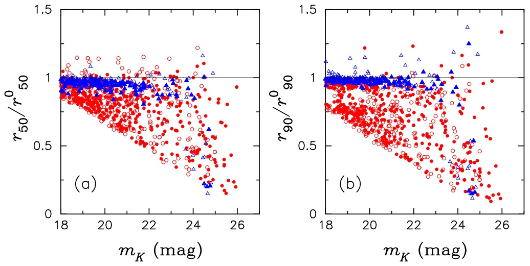
Figure 2: Figure taken from
Ichikawa, Kajisawa, &
Akhlaghi (2012) showing sizes determined from aperture photometry
using SExtractor.
Left -- the ratio of measured half-light
radius (
r50) and model radius
(
r050) compared to the input magnitude
(
mk). One should not take the
x-axis
magnitude numbers literally because it is the signal-to-noise that
really matters. Blue data points are for pure exponential profiles
and red for pure de Vaucouleurs profiles.
Right -- the same
for radius containing 90% of the light. Compare this figure with how
much better parametric model fitting can do
here.
From the above figure, it's clear that aperture photometry produces large
systematic errors at low signal-to-noise (S/N) and when the galaxy profile
is steep (red data points). Furthermore, notice how the systematic errors
for the sizes trend downward, as explained above. To hit home the above
points, what makes parametric fitting a superior technique is that
parametric fitting allows one to test
consistency of the model in the presence of noise beyond our visual impression
of where the galaxy "ends." Again, it is worth emphasizing that
parametric fitting doesn't "see" in the same way that our eyes do.
How do I measure the half-light radius
(re) for a multi-component galaxy, or when the residuals
don't look smooth?
All galaxies are multi-component, so this is a general issue. When
performing parametric fitting to determine the sizes of galaxies, it is not
obvious how to define "size" when a galaxy is lopsided, highly irregular, or
made up of several components. Furthermore, when a galaxy is not very well
fit and the residuals are large, the size measurement can be misleading if
the sky estimate is also affected by the bad fit. Therefore, how does one
determine the size? There are several methods that come immediately to
mind.
- First, even if a galaxy is not well-fitted using a single component,
if the Sérsic is fairly low, i.e. below n~4 and the sky is well
determined, then the size of the galaxy should not be too badly
affected. To check if that's the case, or to try and do a better job,
one can try the following:
- Fit the galaxies as well as possible using multiple components. Here
the goal is not to worry about what the components mean; they may or
may not have physical significance. The goal is to find a set of
components that represents the galaxy light distribution as well as
possible. If any component has a Sérsic index larger than 4
and the residuals are large, then either consider the possibility of
holding that fixed to n=4 or add more components to reduce the
residuals. Otherwise the fit may affect estimates of the sky
background value. If the Sérsic index is high because there's
an extended wing, then additional components will be able to make up
for that. Make sure none of the components have any problems;
problematic parameters will be marked by *...* in GALFIT version 3 and
beyond. After you obtain a good fit, hold the sky value fixed to that
determined by GALFIT, then replace all the components with just a
single Sérsic model: this will let you estimate an
effective Sérsic index and an effective
radius. If the Sérsic index does not behave when doing so,
hold it fixed to a value that yields the same total magnitude
from fitting multiple components.
- Another variation based on the above technique is that, after
obtaining the best multi-component fit, tell GALFIT to generate a
summed model without the sky and without convolving the model with the
PSF. Then, using simple aperture photometry, find an aperture radius
that gives half the total light of the analytic model. This has a
benefit that the "half-light-radius" means exactly what it says,
without subtleties about how well the galaxy corresponds to a
Sérsic profile, and with the seeing properly taken into
account.
What would cause systematic errors in fitting?
GALFIT lets people fit galaxy images in a number of ways, from single
component to many components; from simple ellipsoid shapes to irregular,
spiral, and truncated shapes. Having flexibility is useful for dealing with
a wide range of situations one may encounter. On the other hand, having
flexibility may not be viewed as a good thing if one is worried about
parameter or model degeneracies. Parameter degeneracy is a commonly voiced
concern regarding model fitting in general. GALFIT is constantly being
tested by many people, even 10 years after the first release. Testing
GALFIT is as much about learning the limitations of the code as it is about
making sure the code is being used correctly. For, even if the code works
as it is supposed to, there are ways to use it incorrectly. Over the years,
a number of studies have reported on single and multiple components fitting
tests, and both manual and automated forms of analysis. Based on realistic
simulations discussed in this section and in other refereed papers, GALFIT
seems to work as intended. However, occasionally some new studies report
finding systematic biases that contradict simulations by prior studies.
Some claim that small and large galaxies, bright and faint galaxies, show
different degrees of systematics. Others find that crowded fields can
produce systematic errors. The reason for these behaviors is often
attributed to to parameter degeneracy. However, there are reasons to be
skeptical of such claims. These and other situations are examined in this
section.
The term "parameter degeneracy" means that there are multiple solutions to a
problem that statistically are indistinguishable from each other. However,
the term "degeneracy" has evolved to also mean local minimum solutions, or
generalized even further to mean anything the code does which is not
expected. However, there are many ways for systematic biases to appear in
data analysis yet have nothing to do with parameter degeneracy issues. The
most common examples are situations with neighboring contamination, wrong
sigma image, too small an image fitting size, bad convolution PSF, gradient
in the sky due to flatfielding errors, etc.. To understand where systematic
errors come from and what can be done about them, we have to discriminate
between errors that are caused by things in the data, as opposed to
limitations in the software. Whereas things in the data can and
must be dealt with by an end user (e.g. masking out or simultaneously
fitting neighbors), software limitations mean that there's either a bug
(e.g. pixel sampling errors, internal gradient calculation errors) or there
is a conceptual limitation (e.g. parameter degeneracies, conceptual flaws
in implementation). Before delving into how things in
the data can cause systematic errors, it is worth discussing first the
tests that have been done to verify the software itself.
- Test to check for systematic errors and
parameter degeneracy issues caused by GALFIT:
GALFIT uses a Levenberg-Marquardt (L-M) algorithm to find the best
combination of parameters to minimize the residuals. In numerical analysis,
downhill-gradient-type algorithms like the L-M are thought to not be robust
for finding global minimum solutions. Some people argue in favor of using
simulated annealing or Metropolis algorithms instead. However, there are
many things to consider when deciding "which is better" for galaxy fitting.
For instance, annealing and Metropolis algorithms spend a much larger
fraction of their time, compared with L-M, exploring parameter spaces far
from the best solution, which can mean huge computation cost and which is
why they are much slower than L-M. So in practice the theoretical
advantages may not be easy to realize. There is also a separate concern
about parameter coupling: in galaxy fitting some parameters are coupled, but
being coupled does not mean being "degenerate." If parameters are coupled,
it may not be hard for L-M algorithms to find a vector that descends the
valley of correlated parameters to find a combination which yields the best
solution. And there are few times when the solutions are so close together
in parameter space, or so closely related, that the code can't easily tell
them apart, or that we can't tell which is correct by simply looking at the
results with our eyes. Where degeneracies do occur are in situations where
different parameters describe the same shape, e.g. the axis ratio is
closely related to the Fourier mode m=2. Another situation is when
one chooses to fit fewer number of components than there are actual in a
galaxy, e.g. fitting two components to a galaxy that has bulge + disk +
bar. Doing so results in poor models because the input prior is bad or
simply wrong. No amount of clever manipulation or choice of algorithm
will be able to make up for bad model priors.
In fact, rather than the number of parameters being what really matters, it
is the type of parameters and the situation that matter more.
For instance, a million well isolated stars in the image can be fit just as
robustly as a single star, with no local minima because all the parameters
are decoupled. Whereas a single component fit using both the axis ratio
q and even Fourier m=2 and 4 modes at the same time may have
many mathematically equivalent solutions, even though there are only three
parameters involved. In short, being cognizant about what one is doing
often goes a long way toward undermining supposed advantages of using
annealing or Metropolis techniques, which for galaxy fitting have been
mostly speculated rather than demonstrated, to my knowledge.
Nevertheless, it is important to address some fundamental questions when
dealing with highly complex situations: (1) Can GALFIT robustly fit
multiple component models to find the true global minimum, (2) do so without
introducing systematic biases in parameter measurements, (3) are the final
results sensitive to initial guesses for the parameter values? These
questions are particularly relevant to GALFIT because one reason for using
GALFIT is that it is versatile, but versatility is meaningful only if one
can get right answers. Versatility is needed, for example, to deblend
components, whether in a single object or in crowded environments. This
involves fitting multiple, often overlapping, objects simultaneously.
Although GALFIT has been tested in these regards on an object-by-object
basis, generalizing those anecdotal evidences more broadly is difficult. A
"proof" requires performing industrial-scale image fitting simulations. And
this is only feasible when there is a machinery to analyze large volumes of
galaxy survey data, in an automated way using all the capabilities of
GALFIT. Recently, this has become possible by using a new algorithm GALAPAGOS
(created by Marco Barden -- Barden et al.
2012, MNRAS, 422, 449.), developed in the course of the GEMS project
(Galaxy Evolution from Morphology and SEDs, PI: Hans-Walter Rix, 2004, ApJS,
152, 163).
To test GALFIT on large scale, crowded fields of galaxies, my colleagues,
Dr. Marco Barden and Dr. Boris Hässler devised and conducted many sets
of rigorous simulations using an automated data analysis pipeline (GALAPAGOS,
Barden et al. 2012). The results I'm discussing below come from a paper by
B.
Häussler et al. (2007). Dr. Boris Häussler, whose Ph.D.
thesis partly involved trying to break GALFIT and GIM2D through punishing
use, created the most challenging simulations of its kind to analyze: the
simulations comprised roughly 80,000 galaxies that span the range of
parameters in signal-to-noise, size, surface brightnesses, and axis ratio.
These objects were placed randomly into ACS images (800 per image), as shown
in Figure 3. He then applied GALAPAGOS (a
master wrapping-script that runs GALFIT), which performs object detection
(using SExtractor), extraction, fitting, and lastly, data sorting. The
object densities are quite high: an object has a 50% chance of being
located near one or more galaxies which have to be simultaneously
fitted/deblended (see Figure 3, especially the
left hand panel). And the crowding can range anywhere from 2 objects to 12
objects. To compare the fitting results produced by GALFIT, the same
simulated images were fitted independently by Daniel McIntosh using the GIM2D software. In contrast
to GALFIT, which requires GALAPAGOS for
automation, GIM2D was specifically designed and optimized to perform
automated galaxy fitting, moreover, GIM2D uses the Metropolis algorithm to
determine the best fit.
CROWDED GALAXY SIMULATIONS
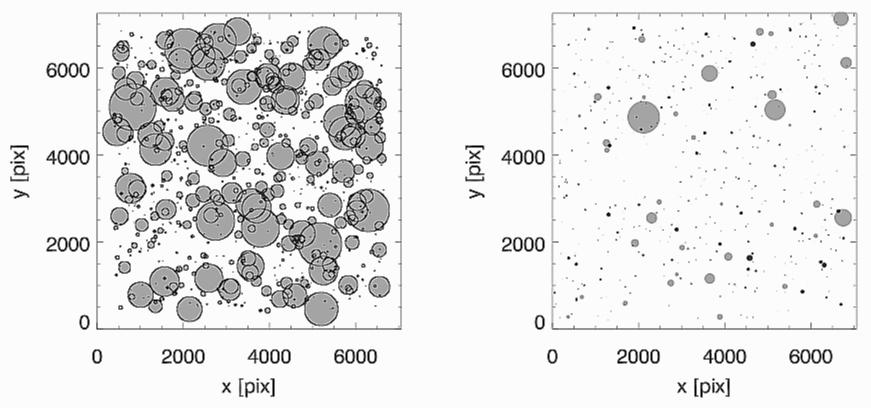
Figure 3: from
Häussler
et al. (2007):
Left -- Crowded galaxy simulations. The
location and sizes (the circles radii = galaxy effective radii) of
n=4 objects in a typical simulated image.
Right --
n=1 (black) and
n=4 (grey) simulated galaxies distributed
like one of the GEMS images, to illustrate the severity of crowding in
the
n=4 simulations.
In Häussler et
al. (2007), they apply GALAPAGOS
(Barden et al. 2012) to analyze galaxy images by using both simultaneous
fitting and object masking, based on whether objects are overlapping or
well separated in an image. Furthermore, hard decisions about which objects
to simultaneously fit or mask out for GALFIT are made in a fully
automated manner so there is no human input once the program gets
going. The fully automated data analysis allows for testing under the most
realistic conditions of galaxy surveys. From these simulations the
following key questions about the robustness of complex analysis using
GALFIT are addressed:
COMPARISON OF INPUT
MODEL RADIUS vs. INITIAL GUESS
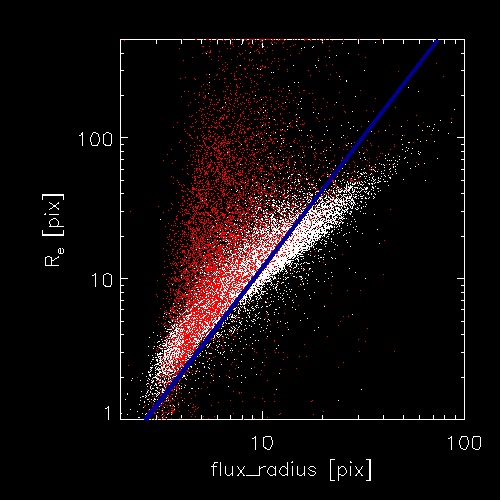
Figure 4:
Comparisons of galaxy radii definitions (courtesy of
Marco Barden). This diagram was used to determine how to
convert SExtractor galaxy radius (defined in some useful way)
(x-axis) into an initial guess for the effective radius
(y-axis) for GALFIT to start iterating on. The red
data points are for de Vaucouleurs (n=4) galaxies
whereas white data points are exponential profile (n=1)
models. The blue line is the input initial guess for the
effective radius into GALFIT. Despite the correlations
between the cloud of points and the solid line, notice the
large difference between the known input model parameters and
the proxy flux_radius parameter, especially for
n=4 models. Then, compare the large scatter in this
figure with the much reduced scatter in Figure 5 below, which shows
simulated vs. GALFIT-recovered values.
- How sensitive are the final
parameters to the initial input guesses? One common concern is
that the final parameters may depend sensitively on initial parameters.
This concern was addressed in Figure 4 which
shows initial input guesses for effective radii, derived from SExtractor
catalog values, compared to galaxy parameters used to generate
the simulation models (Figure 4), i.e. the
correct answer. Clearly there's a huge scatter (the scales are
logarithmic), although there is a correlation. When GALFIT was fed the
SExtractor-derived guesses, it nevertheless converged to known solutions
in the end (Figure 5). So insensitive is
GALFIT to the input guesses that even though some were off by one to two
orders of magnitude, especially for n=4 galaxies, the final
scatter is only of order 0.1 dex. This is all the more striking when
considering the fact that 50% of all the simulated objects have nearby
neighbors, many of which were undetected thus could not be accounted for
at all in modeling or by masking. All the secondary objects being
fitted simultaneously as the primary galaxy also had equally crude
initial guesses for the parameters (Figure 4).
The strong convergence behavior is not just in the effective radius
parameter, but also for all the other free parameters.
- How large are the systematic errors in
the parameter estimates? It is also reassuring that there
appears to be no significant systematic deviation between the
GALFIT-measured and known-input parameters down to galaxies fainter than
three or more magnitudes below the sky surface brightness, as shown in
Figure 5. Around this regime "stealth"
neighboring sources (faint or low surface brightness galaxies) in the
simulations can explain some of the scatter behavior. Stealth sources
can't be removed or dealt with because SExtractor does not recognize
their existence, yet they make up roughly 40% of all sources in the
simulations. Their influence is more noticeable when the primary
science targets are comparably diffuse or faint. At low surface
brightnesses, the issue of sky determination is another which can
sensitively impact the fitting quality. Accuracy of the sky
determination depends on factors like the Poisson noise, flatfielding
errors, the number of nearby stealth sources, and the fitted image size
(which is tied to SExtractor estimate of the galaxy isophotal size, and
which SExtractor often underestimates for low surface brightness
objects). When large numbers of stealthy sources cluster around a faint
primary galaxy, they may effectively act as a non-uniform sky component.
However, even in this quite troublesome regime, it is reassuring that
the measured parameters show little systematic deviations compared to
the size of the random scatter.
- How problematic are parameter
degeneracies? Lastly, comparing Figure
5 with Figure 4 also shows that parameter
degeneracy is not a problem even when large number free parameters and
simultaneous fits are used in the analysis, given that about 50% of all
objects have neighbors which need to be fitted together or masked out.
Furthermore, in all situations where simultaneous fitting is necessary
the initial parameters of all components involved would be
quite crude. If parameter degeneracy or sensitivity to initial guesses
are really that problematic then these are the tests needed to find the
effects. In fact, as shown in Figure 5, the
scatter in GALFIT results for all parameters (size, luminosity,
Sérsic index) compare very well with GIM2D single component
fits. GIM2D
is based on a Metropolis minimization algorithm. In single component
fits for primary galaxies, parameter degeneracy is a non-issue
(see Häussler's
comparison study).
Häussler's study goes to show that object deblending in a fully
automated way not only can be done robustly using a downhill-gradient
type algorithm, and with no systematics if the neighboring contamination
is rigorously accounted, but that doing so is essential for crowded
regimes. The act of masking out objects, by itself, in crowded areas
cannot fully get rid of neighboring contamination that causes systematic
errors in the fit (see Figure 7, in section
on neighboring contamination).
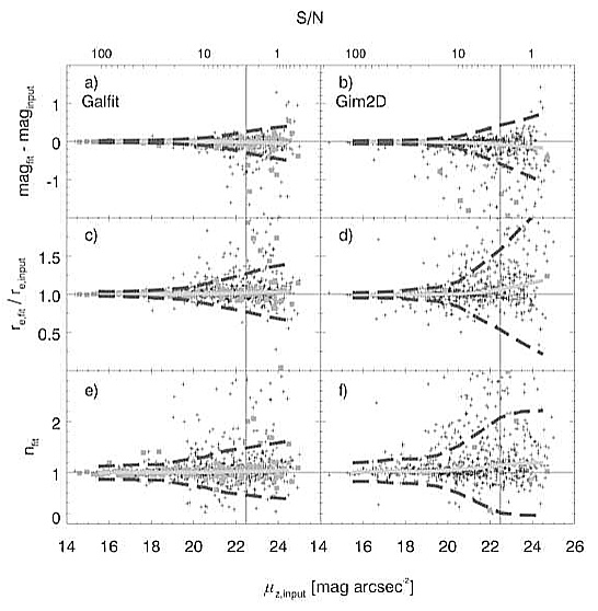
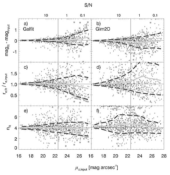
SIMULATIONS OF n=1 (EXPONENTIAL PROFILE, LEFT) and
n=4 (DE VAUCOULEURS PROFILE, RIGHT) MODELS
Figure 5: from
Häussler
et al. (2007):
Top panels -- the difference between
magnitude recovered and simulated values.
Middle panels -- the
ratio of recovered and simulated half-light radius.
Bottom
panels -- recovered Sérsic concentration index.
Top
x-axis -- average surface brightness within the effective radius, in
magnitude per square arcsec. The vertical line is the surface brightness
of the sky level, and the grey line that runs through the data points is
the median of the scatter.
Despite the above tests, users really ought to check for themselves that
GALFIT can do basic things right for their data. Do not take anything
for granted because every data are in some ways different either in the data
processing, in the amount of crowding, or what not. If you should discover
systematic issues inherent in GALFIT itself, and which is not addressed by
the document below, feel free to let me know so I can look into it -- and
thanks in advance.
In literature, there have now been two refereed papers which attributed
some systematic errors to GALFIT. Upon followup communication with the
authors, I discovered that one was caused by the sky not being flat in
their data (which is quite difficult to deal with in some images), and the
other was caused by not properly comparing or using the code (in my
opinion), as discussed here, here and here. Some situations are in fact
very difficult to know about or avoid, even when people are experienced in
data analysis. However, if there are known problems in GALFIT that may
produce systematic errors, it will be quickly updated and brought to
public attention via the main webpage and a user list.
-
External causes for systematic
errors: Even if GALFIT works as it should, there are a number
of situations where systematic errors occur because of something about
the data. This section discusses common situations that users should
be aware of, which are: neighboring
contamination, the wrong sigma image, a
mismatched convolution PSF, using too small a
convolution box/PSF, image
fitting size, or a problem in determining the sky level -- see appropriate links for detail.
For instance, as explained below, neighboring
contamination has the effect of elevating the outer flux regions
around a galaxy, thereby causing an increase in the Sérsic
index, which then leads GALFIT to over-fit the flux and size.
Similarly, an error in estimating the sky value can also make the
Sérsic index misbehave; it leads to systematic errors in
magnitude and size in either direction. Common problems that lead to
bad sky estimation are: fitting too small an image size, a profile
mismatch between the data and model, there being a 2nd order curvature
in the sky due to flatfielding problems or dithering schemes (often
seen in NIR images), or there being neighboring contamination that is
not properly removed. Lastly, a mismatched PSF affects the
Sérsic index in the sense that a broader PSF than normal would
lead to inferring a higher concentration.
The importance of using a correct sigma (weight) image cannot be
overly emphasized. The most natural weighting scheme in a photon
"counting experiment" is Poisson statistics. Changing the definition
of sigma can lead to nicer behavior in some cases, but unpredictable
behavior in other cases. The only way GALFIT "knows" that an object
has high or low signal-to-noise is through the use of the sigma image. Thus a problem with the input
weight map that wrongly weighs bright and the faint pixels can lead to
a bias in the fitting parameters. For instance, a sigma image with a
constant small value would give too much emphasis to the core of a
galaxy, effectively giving the core a higher S/N than normal. This
has the tendency to make GALFIT under-measure the size and luminosity
of a galaxy. Keep in mind that because the sigma in flux goes like
√f , where
f is the count value in unit of [electrons], near the center of
a galaxy sigma should be higher than in the outskirts, even
though the fractional noise (σf / f) (i.e. relative
to the peak flux) is lower in the center.
Users are well advised to spend some time
to familiarize themselves with the concept of a sigma image.
-
SExtractor determined sky value can lead to
systematic errors: One of the common practices in literature
to determine the background sky value is to use SExtractor. Doing so
may adversely affect the fit parameters, which is most noticeable when
fitting the Sérsic profile. The sky value determined by
SExtractor based on thresholding, whereas the sky GALFIT needs is one
based on extrapolating out to infinite radius. Therefore, SExtractor
will always over-predict the sky, the use of which will
suppress the Sérsic index, effective radius, and luminosity.
Häussler
et al. (2007) show that GALFIT determined sky is actually better
than SExtractor determined sky for idealized Sérsic profiles.
This is not a surprise, since SExtractor has no way of knowing where
the galaxy ends. If one finds systematic error in GALFIT analysis, an
immediate questions should be "how is the sky value determined?",
followed by "how is the sigma image determined?"
-
Known systematics in detailed
comparison with IRAF/mkobject models: One of the common ways
for people to generate artificial galaxy models is to use
IRAF/mkobject. Then when they go on to fit those galaxies with GALFIT
they find systematic errors in the fit (more for de Vaucouleurs
profiles than exponential profiles). The differences probably have to
do the fact that GALFIT and IRAF/mkobject generate objects differently
because they are intended for different goals (see following Figure
and discussions). As noted in IRAF/mkobject documentation, the
original intent of the task was to aid photometry (not fitting)
simulations. And for that: "A correction is made to account for
lost light so that aperture magnitude will give the correct value for
an object of the total magnitude" (when referring to the dynamic
range parameter). In other words, the missing outer flux is placed
back into the untruncated part of the profile, which does affect the
detailed profile shape. This is subtly different from fitting, where
no aperture correction is involved, since the total luminosity is
extrapolated out to infinity analytically.
DIFFERENCES BETWEEN IRAF/MKOBJ AND GALFIT MODELS
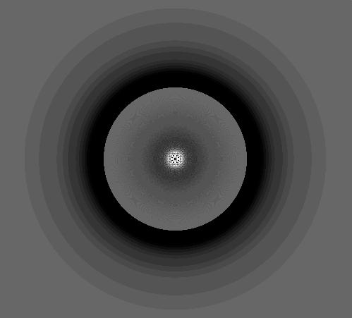
Figure
6: A differenced image of (IRAF/mkobject - GALFIT)
models, in positive grey scale, i.e. white = bright.
The differences in the profiles between GALFIT and IRAF/mkobject can
be fairly large, as shown in Figure 6 on right, depending on how the
parameters in IRAF/mkobject are set (which are stored in
IRAF/artdata). Often times, both codes agree in general but differ in
detail. A galaxy with high Sérsic index (de Vaucouleurs
profile, n=4) will show a larger systematic error than one with
a lower index (exponential, n=1) because high Sérsic
index profiles have steeper cores and more extended wings. The
figure on right, which is a difference between models generated by
IRAF/mkobject and GALFIT (without PSF convolution) illustrates this
clearly:
From the picture it is clear that the biggest disagreements between
GALFIT and IRAF/mkobject are the following: the flux right at the
central pixel doesn't agree, nor in an annulus several tens of pixels
in radius immediately surrounding. IRAF/mkobject appears to create a
profile with pixellated patterns in that region. There's a
discontinuity in IRAF/mkobject profile due to outer truncation (set by
the dynamic range). Just within the truncation, where pixel sampling
differences is not a problem, the residual are slightly more elevated,
due in part to fitting an IRAF/mkobject model that's truncated, and in
part to an effect of IRAF/mkobject aperture correction. The degree of
disagreement varies depending on IRAF/artdata settings, but they never
agree at the central pixel. Unfortunately, it is not easy to figure
out how to set IRAF/mkobject parameters to produce consistent and
reliable agreements to better than 5-20%. Adjusting the sampling
scheme to much finer values in GALFIT produces negligible differences.
To make sure that the problems shown above are not caused by GALFIT,
comparisons were done by several people using different ways (IDL,
MIDAS, GIM2D) to generate or integrate up a galaxy profile. In the
end, they confirmed there appears to be essentially no systematic
errors with GALFIT model profiles to a high accuracy. So no effort
will be made to make GALFIT models agree with IRAF/mkobject.
As a side note: there is a study out on A&&;A early in 2006 which finds
there to be quite significant systematic errors in GALFIT models (see below). On examining what
they've done, it's clear that they used IRAF/mkobject to generate
their baseline comparison models. Their results are also affected by
neighboring contamination and sky fitting issues as mentioned above,
leading to systematics and random errors that are larger than what
ought to be using proper analysis.
- Sampling of central few pixels:
Another issue concerning profile creation is how pixel sampling is done near
the center. High Sérsic index n in galaxies means the central
concentration is very steep. This is because the flux is a high exponential
power of the radius (raised to the inverse Sérsic index), which means
the profile can have a high second derivative within even a single pixel
near the center. When convolved with the PSF, the peak will diminish
greatly in appearance. But, it is still *very* important to sample the
inner few pixels accurately, because the central pixel contains a lot of
flux. This usually means that integration over a pixel has to be done by
numerical integration (i.e. breaking up a pixel into lots of sub-pixels and
sampling/summing the profile variation over that area). If you're creating
your own profiles to check on GALFIT models, please make sure that the
central few pixels are sampled sufficiently finely.
Are 1-D techniques better than 2-D at fitting low
surface brightness regions or irregular galaxies?
- Low surface brightness sensitivity
comparison: It has been argued by some that 1-D fitting
techniques are more sensitive to low signal-to-noise (S/N) or low
surface brightness wings of galaxies than 2-D techniques. Their
reasoning goes that if each point being fitted is derived from
averaging over an annulus, the averaged points have higher S/N
relative to fitting over 2-D pixels directly. However, this is
actually not the case if the weights of the data points come from
Poisson uncertainty, σ, at that point. Whether you first
average over N pixels with similar mean values to obtain
smaller set of points for fitting, or you fit all the points without
averaging, the effective weights are the same, and scale
like: σ<f>/√N
. This is a natural consequence of Poisson statistics.
Taking a step back, given a model that has parameters one can change, χ2, or least-squares fitting
involves finding parameters that yield the lowest value of
χ2. Practically speaking, the quantity χ2 is
simply a way to measure how large the difference is between the model and
the data overall, i.e. Δf = fmodel -
fdata. A model can be as simple as a straight line, to
something much more complicated like an N-dimensional function. Going one
step further, the χ2 used to decide on goodness of fit has a
very specific, i.e. statistical, meaning. It is a ratio of two quantities:
the Δf between model - data, compared with how large a
typical deviation, σ, is supposed to be based on Poisson statistics at
that point. Obviously, the larger the deviation Δf compared to
σ, the poorer is a match between the model and that point, but it is
σ that provides the statistical sense of "bad by how much?" at that
particular point. This idea of maximizing the probability over all data
points, not just one, leads to the idea of minimizing χ2, so
χ2 is the merit function to determine when to stop
fitting. One important observation here is that as far as χ2
statistics is concerned, being a single scalar number, it does not know
whether the data are in the form of a 2-D image or a 1-D surface brightness
profile. In fact, it can careless about the dimensionality of the data,
spatial or otherwise. Therefore it is important to recognize that the issue
of interest here ("is 1-D fitting more sensitive than 2D?") is inherently
not one between 1-D vs. 2-D. Instead, it is about whether it is
better to fit to a few high signal-to-noise points, inferred from averaging
over a subsample of data points to reduce the noise, or to fit all
the data points collectively without averaging them first (assuming here
that all the data points in each bin fluctuate around the same mean).
Because the issue is not about 1-D vs. 2-D, we can simplify the
discussion by referring to a simple example: consider fitting a line
to a set of N pixels that fluctuate around a constant value,
i.e. f(x)=C electrons, over some arbitrary abscissa (x-axis).
A good example is the sky in an image. At this point, the relevant
question is, does the final answer in determining the mean value,
C, depend on how you group the pixels (e.g. fewer vs. more
bins) when doing the fit, if you use up all the data?
The answer lies in the definition of χ2 itself, as one notices
that the denominator is the effective uncertainty
(σi) at each data point
(datai). Specifically, if you average over N
data points around some mean value <f(x)>=C the effective
σeff=<σi>/√N , and the inverse variance
of the mean is:
1/σeff2=N/<σi2>.
Compare this with the form of χ2 equation to notice that
this is exactly the form of the denominator involving
σi, when summed over N pixels with the
same mean. Because of this, χ2 statistics is oblivious
to the exact composition of the data points being fitted, if the error
propagation is done correctly. For a more rigorous exposition of this
topic, please see Numerical Recipes (Press et al. 1997), Chapter 15.
The bottom line is that in least-squares fitting, it doesn't matter
whether the points being fitted are obtained by averaging noisier ones
*first*, or by fitting all the noisy pixels together: they produce
the same result.
Poisson statistics make 1-D and 2-D techniques at least formally
equivalent in the regime where the flux is relatively constant and the
profiles are well behaved in a Poisson sense. However, if the flux
distribution has too high a curvature in an annulus then 1-D
techniques would actually infer a *larger* σ(R) at each radial
point R, making the mean flux less well determined at R. This is
because, in 1-D fitting, the effective sigma[R] must now reflect the
non-Poisson RMS of the flux distribution in the annulus R+/-dR, on top
of the intrinsic Poisson fluctuations at each pixel. This has the
effect of underweighing the central region of a galaxy because of a
larger profile curvature than in the outskirts.
The above discussion does bring up one marginal benefit of 1-D
technique over 2-D. In 1-D fitting, σ(R) is often determined from
pixel fluctuations inside an elliptical annulus -- i.e., once you draw
an elliptical annulus, the RMS fluctuation inside the annulus is your
σ(R), if the gradient is not too steep. This technique entirely
bypasses the need to provide an external sigma image that you need in
2-D fitting. This has one nicety: since the RMS fluctuations may be
non-Poisson, 1-D fitting should, in principle, result in more
believable errorbars than 2-D fitting. However, this observation
sweeps under-the-rug a requirement for statistical independence
between the isophotal rings. In fact, the isophotes are often highly
correlated from one to the next: the current isophote is contingent on
the one that came before. In 2-D, there are clever ways to deal with
this issue, and to create more realistic sigma images, which will be
the subject of future code development.
In summary, a claim that is sometimes heard about the benefit of 1-D
fitting over 2-D when it comes to surface brightness sensitivity is
not correct, from a statistical point of view.
- Fitting
peculiar/lopsided/irregular galaxies: There is another notion
that, because 2-D ellipsoids are not realistic for modeling detailed
shapes of galaxies, 1-D techniques are better for dealing with
peculiar features, irregular isophotes, and asymmetry of real
galaxies. While it is true enough that pure ellipsoids are not
perfect shapes for isophotal twists or irregularities, it is not clear
how the alternatives are "better for fitting peculiar/irregular,
galaxies," or what that actually means. "Better" in what sense?
How does one define the basis for comparison? Without being specific
about what is the benchmark of comparison or what is the "right
answer," it is hard to justify which is better. This section tries to
address the notion of "being better," and will discuss how 2-D fit
results are affected by complex features.
When it comes to comparing how 1-D vs. 2-D techniques do on
irregular/peculiar galaxies, common notions about what better means
are often vague and contradictory. For instance, one thought is that
the technique must be able to (1) break up a profile into different
isophotes, so as to follow the course of isophotal twists and, (2)
average over large numbers of pixels in annuli so as to overcome
perturbations by peculiar features. Thinking more about it, the
ability to track detailed isophotal behavior is only interesting if
the behavior is meaningful. For irregular/peculiar galaxies, as there
is no objective definition for what amount of perturbation constitutes
irregularity, the ability to break up isophotes is moot when
irregularities exist on all scales. There is also a conceptual
problem in the very definition of a "radial profile" itself when the
isophotes may be changing and shifting about erratically in a free
extraction (allowing all isophotal parameters to vary). In such
galaxies the same pixels may be used multiple times, as "isophotes"
overlap through twisting, flattening, or dislocating, so that there
may not be a unique 1-D profile or even a common center for
the isophotes. So, while it is easy to be drawn by the apparent
simplicity and order of 1-D profiles, this simplicity instead hides
away difficult decisions about how to properly extract the profile, or
what the profile means. Thus, when it comes to solving the problem of
peculiar features, the "advantages" touted by 1-D proponents are
mostly speculative. In truth, no one knows how important these
problems are, and, even if important individually, to what extent it
all matters in the end to the science question at hand. Without being
able to define or quantify what is to be achieved, discussions about
which method is generally better for arbitrarily peculiar systems is a
bit circular.
It is clear that to know what "better" means, a goal has to be well
defined. And the bottom line for most people when they do profile
fitting is to obtain a set of simple numbers, for instance,
luminosity, size, concentration, and to much lesser extent the axis
ratio, position angle. In terms of those principle parameters, the
interesting fact is that there are *regularities* in most
galaxies. Indeed, that is the main lesson gleaned from 1-D profile
extraction. Even in irregular/peculiar galaxies, three of the
regularities are: they have an average size, an average profile which
falls off with radius, which, by definition, has some kind of average
"center." Indeed, the notion of "average" is the key,
such that over sufficiently large regions even irregular galaxies have
well behaved properties. It's not hard to convince oneself of that --
all one has to do is smear out an irregular galaxy image modestly with
a Gaussian. It is this averaged regularity that is often of interest,
and it is precisely because of this averaging sense that 2-D fitting
using ellipsoids (which, fundamentally, is a weighted *average* over
an elliptical kernel) doesn't do such a bad job, despite the
shortcoming of its shape. It is also why detailed information about
isophotal twists obtained in 1-D extraction does not have as large an
impact as one might surmise. Nonetheless, it is true, as 1-D
proponents argue, that the ellipsoids having a fixed center, makes
traditional 2-D fitting rigid, which might then affect an estimate of
the central concentration and slope of a galaxy, even if the size and
luminosity, on average, are O.K. (as enforced by least-squares
fitting). But, while 1-D proponents argue this to be a problem,
exactly *how big* has never been shown because "compared to what"
has never even been defined. Nonetheless, the answer is actually not
much, as will be argued (but not rigorously) below. And to the extent
that galaxy morphology is a messy business to begin with, and even
more so for irregular galaxies, 2-D algorithms are probably O.K. in
an average sense.
To quantify what O.K. means we have to define a comparison baseline.
There are several ways to do this. But the baseline should not be to
use 1-D profile results as ground "truth" if the goal is to test
whether 2-D is more robust than 1-D (there has been one study in
literature which used this circular argument that one should be aware
of). Instead, what is more interesting to see is which one is more
internally consistent. This kind of comparison is very much beyond
the scope of this FAQ and I will not do so here. Instead, I
illustrate that 2-D, bland, ellipsoids don't do too badly even on
rather irregular-ish galaxies compared to a much more sophisticated
technique.
To do so, a much more complex fit is performed by GALFIT Version 3.0 which will be used as the
baseline. GALFIT 3.0 will allow 2-D algorithm to break from
axisymmetry completely, while retaining the useful traditional
parameters such as effective radius, Sérsic index, axis ratio,
and the ability to decompose multiple components. Many such examples
are shown here. But, the main point is
that 2-D fitting is not limited to using
ellipsoids. In fact, 2-D fitting can be extremely realistic,
with lopsidedness, spiral structure, and so on. (Which, by the way,
also defeats another common argument against 2-D fitting in preference
over another.)
However, for the purposes of this section, I will illustrate by way of
three examples why ellipsoids are "not that bad." The three
examples are VII Zw 403, NGC 3741, and II Zw 40, which are found here. These examples show that despite the
irregularity and complexities that are involved, a single component
(except for II Zw 40) using new features does a rather nice job at
tracing the general galaxy shape (lopsided, peculiar, or otherwise).
Now, when a traditional ellipsoid is fitted to these galaxies, the
differences in size, luminosity, and the Sérsic index values
are about 2-5% -- all except for the extreme case of II Zw40, which
has an error in size by about 15%. Having now fitted many
irregular-looking galaxies, this trend appears to be fairly
representative of the differences between naive ellipsoids and more
sophisticated 2-D fitting on peculiar/irregular galaxies. Therefore,
in terms of *internal consistency* 2-D techniques using traditional
ellipsoids are not bad at all, even on galaxies of questionable
propriety for using ellipsoids.
Are 1-D techniques more robust against neighboring
contamination than 2-D fitting techniques?
There are often discussions about whether 1-D fitting, or some hybrid scheme
combining 1-D with 2-D, is more robust against neighboring contamination
than 2-D fitting. There is even one study years ago which claims that 1-D
analysis, or a hybrid scheme is better. However, after examining the claim
closely, it seems like the results came from not treating 2-D analysis in
the same way as in 1-D analysis. I am aware of no other study which finds
that 1-D techniques are more robust, nor less so, against neighboring
contamination. But if common sense is a guide, it would argue that 1-D
techniques ought to be
less robust, as discussed below.
It is worthwhile, first, to consider why it is surprising and
counter-intuitive to claim that 1-D techniques are superior or more robust,
with all else being equal (experimental factors such as image fitting size,
masking, etc.). How well 1-D analysis can be done depends on how well 1-D
profiles can be extracted from 2-D images. If a galaxy is embedded in a sea
of background sources common sense would say that 1-D techniques have no way
to rigorously deblend a neighboring galaxy, and the only recourse is to use
"masking." But masking only goes so far, and cannot remove light which
continues to extend beyond the mask. Therefore, the more crowded an
environment, and the fainter an object of interest, the more problematic is
neighboring contamination for extracting a 1-D profile. In fairly crowded
limits, no amount of masking would do without blocking out the whole galaxy
one is interested in fitting. As explained below, image fitting is especially sensitive to
neighboring contamination because galaxy wings can be highly extended, which
is one reason why sometimes accurate sky determination is difficult
but very important. As also discussed above,
both 1-D and 2-D techniques are equally sensitive to the faint extensions of
galaxy profiles. Furthermore, Figure 7 clearly
shows that object masking alone does not suffice to remove the influence of
neighboring contamination, the extent of which depends both on the
luminosity and distance to a neighbor. Since accurate treatment of
neighboring contamination is key for obtaining accurate results, it would
seem sensible that a 2-D technique might be beneficial for this reason. In
2-D fitting, nearby neighbors can be simultaneously optimized and fitted to
remove the contamination that can't be masked out. Indeed, detailed, crowded, simulations of over 40,000
galaxies, and Figure 7, suggest that
simultaneously fitting the neighbors, coupled with masking, is definitely
more robust compared to no treatment of neighbors or only using object
masking alone, especially when there are multiple neighbors which need to be
simultaneously fitted.
Therefore, where had the notion that 1-D fitting methods being more robust
than 2-D techniques come from? Here are some instances that have caught my
attention -- errors which one should be particularly aware of to judge
claims of that sort:
- Baseline models and mixing of systematic
error sources: At one time, it has been common to use
IRAF/mkobject to generate baseline galaxy models for comparison.
However, doing so produces galaxies that have known systematic problems. These
systematics can be fairly significant when fitted by 2-D codes, and
the extent depends on the Sérsic index n. These
systematics would not appear in 1-D fitting tests as the claimants
relied on using IRAF/mkobject to create their models. Also, the
systematics are higher for larger Sérsic index n.
Therefore, when people found that 2-D analyses had larger scatter
compared to 1-D, it was because they combined n=4 and
n=1 simulations without removing the systematic errors between
the two models.
- Using masking for 1-D profile extraction, but
not for 2-D fitting: Another issue which has been a problem
when comparing 1-D and 2-D analysis was what to do about neighboring
contamination. One study has chosen to mask out neighbors using SExtractor
to remove neighboring contamination when extracting 1-D galaxy profiles -- a
perfectly sensible thing to do. However, when they performed the analysis
using 2-D fitting, they did not apply the same treatment. Object
contamination is indeed a serious problem for both 1-D and 2-D fitting, as discussed in the following FAQ. But results from
this kind of study can be understood as an unequal treatment of the two
different algorithms.
- 1-D vs. 2-D fits to real galaxies were
compared against "truth", as defined by other 1-D fits: When it comes
to fitting real galaxies, there is no a priori way to know what in
fact is the true answer. That is why idealized simulations are the
necessary first step in every analysis. For real galaxies, a
baseline for comparison, i.e. the "ground truth", has to be defined
for 1-D vs. 2-D comparisons to have any real meaning. One particular study
has chosen as that baseline "truth" to be other 1-D studies. Doing so
misses the fact that there may be fundamental differences between answers
provided by 2-D and 1-D codes. 2-D codes may not agree with 1-D codes if
there are isophotal twists, perturbations, lopsidedness, asymmetry, even in
the complete absence of neighboring contamination. Moreover, it is expected
that comparison of the same types of codes, e.g.1-D vs. 1-D, or 2-D vs.
2-D, techniques should be more internally consistent than across
different types, i.e. 1-D vs. 2-D. Thus, the fact that 1-D vs. 1-D
comparison results in as smaller scatter than a 1-D vs. 2-D comparison
should come as no surprise, and does not indicate better robustness of 1-D
codes against contamination/peculiarities.
- A belief/assertion that, in 2-D fitting, it
is impossible to trust simultaneous fitting results (therefore not bothering
to try): In one particular study, the author admits that, "In the
above comparisons, the performances of both GALFIT and GIM2D were
artificially lowered, since we forced them to model the galaxies with a pure
Sérsic law, while both were optimized to be used with multi-component
models." Then, they assert, "On the other hand, using such models involves a
large number of free parameters, thus making the tool extremely sensitive to
the choice of the initial guesses of the parameters themselves." In
practice, that assertion is not well founded and and has even been shown not
to be true based on actual practice on highly complex
simulations. The reason dire fears are rarely realized is that the vast
majority of objects are spatially resolved, even if overlapping. In those
circumstances most degeneracies are broken. Even if some degeneracies
remain for real galaxies, it is often better to roughly account for
contaminating light than to not account for it at all. It is therefore
highly advisable to use both masking and simultaneous fitting in crowded
field analysis.
Why are the fit parameters so sensitive to the
sky value and/or the presence of neighboring galaxies?
- This is a well known issue in the galaxy fitting business that one
should be very cautious about. Galaxy profiles can decline very
slowly out at large radii. In fact, for normal galaxies, the more
centrally concentrated a galaxy is, i.e. large Sérsic index
n, the more slowly the outer galaxy wing tends to decline
(sounds paradoxical, but that's how the function is defined). Because
of this dual behavior, having elevated flux in the outskirts due to
contaminating sources (i.e. galaxies, flatfield errors, etc.) can
sometimes lead to a higher than normal Sérsic index n.
For this reason it is important to be aware of the flux profile in the
wings, and also to get the sky value right. If a profile already has
a high intrinsic Sérsic index (n > 2), a small error in the
background sky can drive the index up even higher, leading to large
systematic errors in the magnitude and size. This means that a de
Vaucouleurs profile (n=4) is highly sensitive to neighbors,
while an exponential profile (n=1) is significantly less so.
NEIGHBORING CONTAMINATION ON GALAXY FITTING
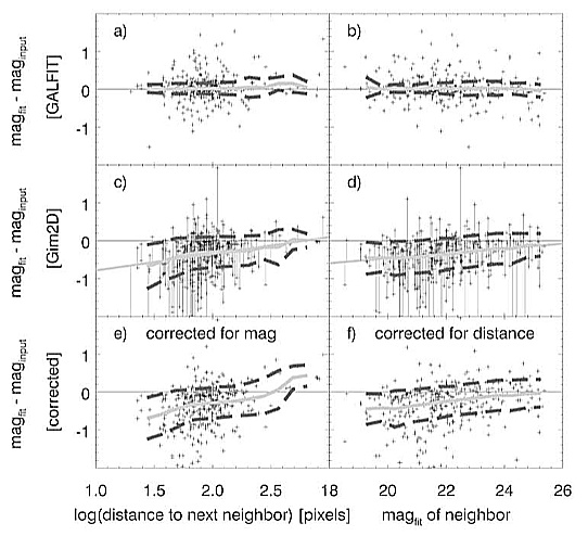
Figure 7:
How neighboring contamination affects the recovered
galaxy luminosity, from Häussler
et al. (2007). Top panels -- GALFIT simulations,
showing that the magnitudes can be recovered reliably when
neighbors are fitted away simultaneously as the primary
targets. Middle panels -- GIM2D simulations, using
object masking to reduce the influence of neighboring
contamination; systematic errors remain even so. Bottom
panels -- GIM2D simulations, after subtracting the median
values from the Middle panels ex post facto.
Figure 7, shown on right, shows an example of the effects of
neighboring contamination on galaxy fitting, taken from studies by Häussler
et al. (2007). Figures 7a-b show that if neighboring objects are
properly accounted for (i.e. fitted together), then galaxy
luminosities can be reliably recovered. However, Figures 7c-f show
that if only masking is used to blot out neighboring galaxies from the
fit, there would be systematic errors that depends both on the
proximity and luminosity of the neighbors.
- Galaxies are generally not represented perfectly by the
functions being used to fit them. If there is a profile mismatch, the
sky level might change to try and compensate, the result of which is
that the sky may take on unrealistic values. The most common
situation is for the Sérsic index to grow out of control, which
then suppresses the sky parameter value. In this scenario, the galaxy
would appear bigger, brighter, and more concentrated than if the sky
were held fixed to a known value. But if the sky is held fixed to
some known value, the growth of the Sérsic index can be
kept in check.
- The important thing to keep in mind is that an
over-estimated sky will generally produce a lower Sérsic index,
a fainter luminosity, and a smaller radius (they are all connected).
An underestimated sky will, of course, have the opposite behavior. Be
also especially cautious if the sky has a high order curvature, i.e. a
2-D parabola, saddle, etc., as higher order sky curvatures aren't
modeled. That can cause weird systematics. This has been seen in at
least one publication, Longhetti et al. 2006, (astro-ph/0610241)
using NIC2 data. In their defense, not a lot can be done about the
fact that the sky has a curvature in the NIC2 image (which they are
kind to provide me), apparently caused by amplifier glow and a
flatfielding issue, which caused GALFIT to overestimate the sky.
Holding the sky fixed to more representative values away from
artifacts, the fit does come out without weird systematics, but that
relies a bit on already knowing the answer.
- Suggestion: Do not fit the sky if
you can estimate it accurately. But, if you choose to do
so.... If the image is only about 2 to 3 times visible size of a
galaxy, the sky fit may still not be reliable. Even if the image is
significantly larger, seriously consider holding the sky value fixed.
To fit the sky accurately the image should be much larger than the
visible wings of the galaxy. And always keep in mind that the sky
determination becomes increasingly unreliable the larger the
Sérsic index n becomes for a galaxy.
- Using sky values determined by
SExtractor for galaxy fitting can lead to systematic errors:
To see why, go here.
Is it sometimes better to use uniform
(or another non-Poisson) weighting scheme in the fit?
Sometimes a discussion comes up about whether it is better to use
"uniform" weighting scheme instead of Poisson weights. The lead-in into
the discussion is usually a belief based on observations that, in plots of
1-D profile, one part of the galaxy, like the outer region, doesn't fit so
well, seeming as though the code "does not see" that part of the galaxy.
This seems to make intuitive sense from a statistical standpoint in that,
as some reason, 1-D codes are more sensitive to flux in the outer region
because each data point is derived by averaging over a lot of pixels,
whereas 2-D algorithms work on low signal-to-noise pixels in-place. This
erroneous understanding of statistics leads one to conclude that the outer
region should be given a bit more weight than the inner region of the
galaxy. This issue comes up in discussions about the merits of 1-D vs.
2-D analysis and, as explained
in this
section, the notion that 1-D data have higher signal is based on a
misunderstanding of how statistics work. For, there is no more
information in a 1-D surface brightness profile than there is in a 2-D
image. However, what is true is that 1-D surface brightness fits and 2-D
fits may not always agree, but that is not caused by
the weights.
Rather, the difference comes from the process of extracting a 1-D profile,
which
loses spatial information content compared to analyzing a 2-D
image.
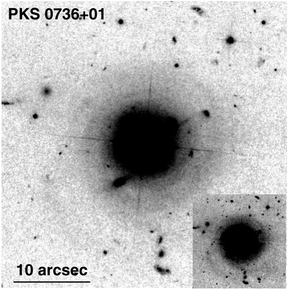
Figure 8a:
Image of quasar PKS 0736+01, from Bennert et al. (2008, ApJ,
677, 846). Original data from the Hubble Space Telescope showing the
quasar+host galaxy and the surrounding area. The inset shows the same
image but with a deeper stretch.
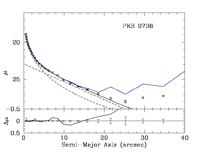
Figure 8b:
This surface brightness profile is constructed by first
fitting the data image in 2-D (Poisson weighting), then 1-D
profiles are extracted in some way, e.g. by running IRAF/ellipse
on the 2-D images of the data and the model independently. The
fit is not done in 1-D; it is only a visualization. The square
points are extracted from the data with some pixel masking, the
dashed lines are the bulge and disk model components, whereas the
solid line is the sum of the two components. The lower window
shows in more detail the disagreement (difference) between the
data and the model. The blue line is the galaxy profile if there
is no mask used.
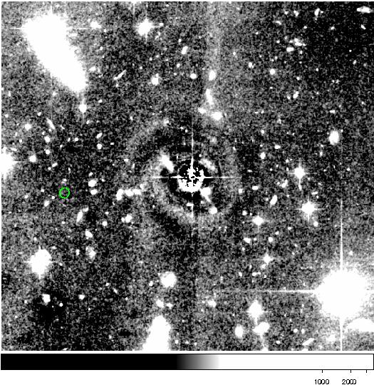
Figure 8c:
The residual image corresponding to the surface
brightness profile plot of Figure
7a (in the spacecraft orientation).
Here's a specific example (see Figure on right) taken from a work I did
with Profs/Drs. Vardha Bennert and Gabriela Canalizo (2008), where the
brightness profile is that of a galaxy
hosting a luminous quasar. When the central quasar and the galaxy are
removed, this is
what it looks like. The
1-D plot (
Figure 8b) shows a clear excess
in the outer region (beyond radius of 20 arcsecond), compared to what the
model looks like when the object is fitted in 2-D, shown in solid black
line (the dashed lines sum up to yield the solid). Clearly, the 1-D
profile data points (in squares) show an excess of flux in the wings
compared to the model shown as a solid line. Because the analysis is done
in 2-D, and only visualized in a 1-D plot, this is often interpreted to be
evidence that 2-D analysis places too much weight to the central region
(due to higher signal-to-noise there) at the expense of the outer wings.
So some people hypothesize that weighing all the pixels uniformly in the
image would solve the problem by shifting the weights more to the outer
region.
If you were to do the analysis using uniform weights, indeed, it
does seem to produce the desired effect of reducing the outer wing
residuals, as long as the data are displayed as a 1-D plot. So what's
wrong with believing that giving uniform weights means the outer region has
higher weighting?
It might surprise most people to hear that, quite contrary to their
belief, weighing all pixels uniformly actually gives higher weight to
the bright central regions of an image in 2-D fitting. The
explanation for this statement is most easily seen from the definition of
the χ2 equation, in which the
weight sigma, σ, is on the denominator. The larger the sigma,
therefore, the smaller is the weight. So if you don't want a fitting
algorithm to "see" a pixel, you make σ really really large for
either that pixel or a region of an image. That region then contributes
zero value to the χ2 sum. Making all pixels have uniform
weights increases the importance of the bright pixels relative to
faint ones by a factor of (flux_bright/flux_faint)2 compared to
Poisson weights.
So then, why does making all weights uniform produce a more desirable
fit to the wing of the galaxy, at least to the eye in 1-D plot? One
of the two main reasons for this behavior is exactly that when more weight
is given to bright pixels the central region is better fit than outer
regions. This causes the sky (which is also fitted as a free parameter)
to be elevated to a higher value, because the sky has one degree of
freedom that can be used to minimize the residuals in the inner region.
In 2-D fitting, this causes the wings to be over-subtracted more than
Poisson weighting, thereby artificially truncating the galaxy profile; in
the extreme that the outer points don't matter at all, the effect is the
same thing as reducing the image fitting region. Now consider the process
to extract a 1-D profile from a 2-D image: one has to first subtract out
the sky -- the sky that you remove is now a higher value than before,
which makes the 1-D profile "look" like the fit got rid of the wing
better, but not for the reason you think. The second reason is
psychological: that most often when the data points (square points) lie
above the model fit in the wings as shown in Figure
8b (solid line at R > 18 arcsec) people will judge this to
be evidence that the central region is over-weighted, because, as they
reason, the model does not "see" the flux in the wing. Whereas, if the
data points were to lie *below* the model, our inclination is to explain
away the disagreement as there being a "break" in the exponential profile
due either to tidal truncation or spiral arms: therefore the disagreement
seems less troubling. Indeed, the upshot is that when there is excess
flux in the wings, people usually consider the problem to be in the
weights, but less so when there is a deficit.
But, doesn't the bottom line that the agreement *seems* better between
the 1-D profiles argue for using uniform weights? The answer is still
no, and we now discuss why by asking the following question.
- Is the disagreement between 1-D surface brightness profiles of
the data and the 2-D model fit really a problem with 2-D fitting, or
with the 1-D profile extraction? While the answer might seem very
obvious (for, how can the data extraction be "wrong"?), a closer look
at 1-D profiles of Figure 8b will
reveal why the problem is with 1-D extraction: the blue line is the
galaxy surface brightness profile when neighboring objects in the
image are not properly masked out, whereas the square, discrete, data
points are the profile with some amount of masking. After masking, it
is clear that the excess wing drops considerably, but apparently not
completely. So it is not hard to believe that at least part of the
discrepancy between the data and the model may be due to incomplete
masking.
Still, it begs the questions: why shouldn't GALFIT fit that excess
flux by raising the sky further to achieve a better fit? The
answer is that a "better fit" in 1-D can actually be a worse fit in
2-D. Sounds crazy, but read on. In Figure 8c, on right, I show an image
where the target of interest, originally at the center, has been
subtracted out, so this is a residual image corresponding to the
surface brightness profile shown in Figure 8b. From Figure 8c, it is clear there's a lot
going on -- there are many neighboring galaxies and stars, which are
discrete and localized as opposed to being the diffuse emission from
the central galaxy, so their profiles can't be modeled if they are not
fitted simultaneously. Often times, the way to deal with neighboring
contamination is to use masking, as it was done in this case.
Nevertheless, it is quite hard to do so fully, especially at large
radii where the contaminations are due to quite extended objects. For
comparison, there is a small green circle located about 30 arcsec to
the left of center of the image (find this radius also in the surface brightness profile above). The
circle encloses a region where the average sky brightness is roughly
zero counts. That is to say, areas of the image darker than inside
the green circle are over-subtracted, whereas regions that are
brighter are under-subtracted. In 1-D profile, the reason for the
rising profile beyond 18 arcsec is that the neighboring objects
contaminate the wing of the primary object at the center (now
removed). Therefore, in 2-D analysis, raising the sky value to fit
the neighbors will in turn over-subtract a much larger portions of the
image of the real sky . In such a situation, GALFIT will
always over-subtract the image because the fit is done in 2-D.
Whereas, displayed in 1-D, the profile will show an excess, depending
on how the pixels are rejected and averaged in the extraction.
From this image, it is then intuitively obvious why GALFIT cannot
extend the wing of the exponential disk component to "better subtract"
larger regions: because doing so would over-subtract a much larger
region of the image to try and account for neighbors which are not
part of the object of interest. The information about whether the
"excess" flux in the outskirt comes from the galaxy of interest, or
due to neighbors, is completely lost in 1-D profiles. Because
of the spatial information in 2-D, and because 2-D models use strong
priors, i.e. that the shapes (ellipticity, PA) of the host galaxy
profile are concentric and radially declining, the fitting
algorithm can more effectively "deduce" whether the contamination is
due to the primary or neighboring objects above and beyond simple
masking alone.
So the main point is that a disagreement between 1-D profile and
2-D model is not always evidence of a poor fit in 2-D: 1-D
profiles are obtained by averaging over all radii, where bright
neighboring galaxies have disproportionately large contributions when
the surface brightness of the main galaxy out there is low. Whereas,
in 2-D fitting, contaminating galaxies at large radii from the primary
have only so much leverage on the profile because it is constrained
also by the shape and orientation parameters. This, in principle,
produces a more realistic fit, and is one of the virtues of 2-D
fitting compared with 1-D. This sounds quite a bit like saying that
the model is better than the data at determining what is right.
However, keep in mind that the 1-D profile depends on the sky
subtraction. So in some sense, 1-D profile of "the data" is not pure
data -- it is model dependent on how exactly the isophotes are
extracted from a 2-D image.
The bottom line is that the only way to know whether Poisson weights
are a problem is to produce simulations to make sure that there are
not systematic biases in situations similar to that shown in Figures
6. This is discussed in the section on
systematics of galaxy fitting. It is one of the reasons for not
preferring uniform weighting to Poisson weighting, even when there is
quite significant object contamination.
- What about other weighting schemes besides giving every
pixel the same weight? The trouble with going beyond Poisson
weighting is that what scheme to use becomes more subjective. We know
that in the limit of low signal-to-noise, that scheme has to converge
toward Poisson weighting because photon statistics dominates.
Therefore, that alternative weighting scheme has at least three free
parameters, the transition point to Poisson dominance, the
normalization of the scale, and how non-linear is the mapping from
counts to weights. While some schemes can be contrived to optimize
for some situations, they will fail for the opposite scenario
that scheme optimizes for.
What fitting box size should I use?
- To decide on a fitting box size one has to consider the
science goal. There are some instances where the accuracy of the
parameters is not important, in which case the box size can almost be
arbitrary. However, most of the time the fit parameter values do
matter, so the image size has to be significantly larger than the
object or component one is interested. The box size is highly object
dependent as well: for instance, an elliptical galaxy has a much more
extended envelope, extending well beneath the noise level (but still
significant due to the large number of pixels), than a late-type
spiral or irregular galaxy. Therefore, to the extent that GALFIT is
**much more** sensitive to our eyes for low surface brightness
features, deciding on a box size depends on trial and error at the
start, and, with time, on one's own intuition/experience. This means
that an iterative technique rather than a rule of thumb should be the
guide for determining the fitting box size, thus I suggest the
following.
Suggestion: try starting out with an image diameter at least twice
the diameter of the galaxy. Once the fit converges, enlarge it to a radius
2-3 times as large as before. Once that converges, enlarge the box once
more to something like 2-3 times larger than that. The reliability of the
fit, of course, is tested by seeing that the parameters stop changing much
with growing fitting area. If the fitting parameters continue to change
significantly with increasing fitting box size, then the cause has to be
tracked down. If the image is already very large but the parameters keep
changing, that usually means there's a significant profile mismatch, which
is causing the Sérsic index to misbehave, or there's significant
neighboring contamination. A typical solution is to hold the sky value
fixed in the fit, or to mask out the neighboring contamination.
- From this discussion, it should be obvious that if you're
interested in the global galaxy parameters, and you want to *fit* the
sky as a free parameter, then the fitting region must be considerably
larger than the visible diameter of the galaxy. It certainly has to
be larger than if one were to consider holding the sky fixed. Again,
it is worthwhile to grow the fitting box to see if the solution
changes much.
What convolution box size should I use?
- In general, the steeper the inner galaxy profile and the
broader the PSF, the larger the convolution box size should be. As a
rule of thumb, I always use a convolution box diameter at least 40-80
times the FWHM of the PSF seeing disk. Sometimes the wing of a PSF
can be highly extended even if the core is very sharp (so don't be
deceived) -- for instance, even though an HST NIC2 PSF in F606W is
Nyquist sampled (i.e. 2 pixels in FWHM), there is still a significant
amount of flux out to a radius of 128 pixels. For fitting small
images GALFIT is fast enough that even using a convolution box 40-60
times the PSF FWHM won't slow one down too much. Like with the fitting box size, one should try an
iterative approach to determine the convolution box size, making sure
that the solution is not much affected by the choice.
- One should keep in mind that for fitting boxes smaller than
than a few hundred pixels in length, convolution takes up at least
half the time in the fitting process. Suggestion: Usually,
at first you'd just want to "hone in" on an approximate solution
quickly. So a good way to start is to go with a small convolution
box. Once the solution converges, get a more accurate solution by
refitting with a large convolution box.
How do I create a point spread function (PSF)
for convolution?
Creating a point spread function (PSF) is not difficult, but creating a
good PSF can be rather subtle and occasionally technical. When you
think about a PSF, the picture that should come immediately to mind is a
bright and isolated star, with nothing else around, and with no sky
background. It is useful to understand that the PSF, technically, is an
image of a perfect point source rather than "just an image of a star"; it
is how a perfect point is transformed into an image by reflecting and
refracting optics and other media (e.g. atmosphere). In astronomy, we
only care about far-field PSFs, where the wavefront from a point source
impinging on the primary mirror of a telescope comes from infinity, and is
in principle flat, as opposed to having a high curvature for near-field
PSFs. That far-field PSF wavefront may not be perfectly flat if it has
passed through an atmosphere, or some other refractive medium, before
getting to the telescope. The PSF that observers usually care about is the
overall PSF from light that has gone through the atmosphere, the telescope
optics, and whatever else before or in between. That's the reason why when
we talk about a PSF, most of the time we mean an image of a star. However,
the PSF may very well change with time and physical location on a detector.
A PSF is not just a property of the telescope; it is a property of every
scattering and refracting interstellar and atmospheric media, as well as
all telescope and reimaging optics in between the emitting point source at
infinity and the detector.
A PSF can be obtained from an image or from from a theoretical model, or
some combination thereof. A theoretical model can be simple, like a
Gaussian function. Or it can be quite sophisticated. For example, if one
were to analyze data from the Hubble Space Telescope, the theoretical models
are made by a program called TinyTim.
However, for high contrast analysis (e.g. quasar host galaxies), theoretical
PSFs are usually not ideal because the profile may not be realistic, or the
PSF of the data may change with time and position on a detector. So ideally
one should prefer to extract PSFs empirically from the data images (which
have also undergone the same image processing that may distort the PSF) over
using theoretical models. However, doing so from data is not always easy
because there are usually few, if any, stars that are bright, unsaturated,
or isolated. Therefore one often has to make do with faint stars, or come
up with a hybrid technique that combines analytic models with empirical
data. For instance, if there are only faint stars, it might possible to
create a high quality PSF from the data by adding them up to increase the
signal-to-noise (S/N). Or one can also fit analytic models to the stars
themselves and use the analytic model as the PSF which would then have
infinite S/N. A third way would be to take a theoretical model, and
convolve it with one or more functions to try and match the faint stars in
an image. The details of how to do so will be explained below.
-
WHAT IS AN IDEAL PSF?
An ideal PSF has all of the following criteria:
1. Isolated from everything else: The PSF has to be isolated
from any and all sources of contamination, including other stars,
galaxies, detector artifacts or defects of negative and positive
residuals alike. If any of these things exist in a PSF image, they
will show up again, often even more strongly, when the model is
convolved with the PSF, and that is often undesirable and may have
weird consequences.
2. Very high signal-to-noise (S/N)-- ideally, infinite: The
S/N of the PSF should ideally be infinite, otherwise, when the PSF is
convolved with a model, the result will look noisy. This may affect
the quality of the model fit. The technique section just below will
explain how to obtain a PSF with infinite S/N.
3. Flat and zero background: The background has to be flat
and zero in value, i.e. the sky background has to be removed and
cannot have a gradient, blotches, weird moire or other patterns. If
any of these things show up in a PSF image, they will also show up in
the model image when it is convolved with the PSF. A PSF image that
has a non-zero sky background will show a "jump" between regions
inside and outside the convolution box, and will affect the fitting
parameters.
4. Should match the detailed shapes of a stellar image, including
things like ellipticity, diffraction rings and spikes, extended halo,
speckle pattern, etc.: This means that if you subtract a PSF from
an image of a field star, there should be nothing left over except for
noise. This is both a statement about how to construct a PSF as it is
about how to check if your PSF is a good one: go and do a
model subtraction! Keep in mind that if there is significant
geometric distortion across an image, the PSF will be position
dependent. If you can't obtain a high S/N PSF from an image, the next
best thing is to match the full-width at half maximum (FWHM) of the
stars.
5. Be correctly centered in the image: The peak of the PSF
needs to be centered in a specific way described below. If it is not,
when the model is convolved with the PSF, the flux centroid will
appear to be shifted relative to the (x,y) position that GALFIT
reports, because of the convolution theorem. This shift will only
affect the part of the model that lies within the convolution box; the
region outside the convolution box will not be affected. To center
the PSF correctly, follow this guideline:
How to center the PSF: If the
number of pixels, NPIX, along an axis (row/column) is odd (NPIX=odd),
the PSF peak should be centered at NPIX/2+0.5, where NPIX is the
number of rows/columns along a side; if NPIX = even, at NPIX/2+1. The
PSF image can be rectangular.
6. The image of the PSF should be sufficiently large to contain
all the light, but not gratuitously large: The image of the PSF
should be large enough to contain 100% of the light. If the PSF image
is so small that it cuts off the wing of the PSF, two things will
happen. First, the model image will show a "cliff," where the wing
of is truncated. Second, the flux of the model will be in error by
the fraction of light that is cut off. However, don't go overboard
and generate a PSF image that is gratuitously large, because doing so
will slow GALFIT down greatly because image convolution is one of the
biggest bottleneck in fitting. The rule of thumb is to start with a
small PSF when you're trying to figure out what models to use, how
many, what combination is best, etc.. This may take several tries.
Then, once you obtain a solution you think is final, that's when to
use a larger PSF to redo the analysis one last time to get the fluxes
and detailed profile shapes right.
The key to figuring out "how big is big enough" for a PSF image is to
try wider and wider PSF images until the result of the fits no longer
depend on the PSF size. That usually happens somewhere between 20-50
times the FWHM of the PSF (there's a lot of flux out there). That
means a typical PSF image is between 50 to 100 pixels on each side,
but may be larger sometimes -- always check!
7. Nyquist sampled: This means that that the full width of
the PSF at half the peak, i.e. FWHM, should at least be 2 pixels or
wider. Sometimes, the data image itself might not be Nyquist sampled,
in which case obtaining a Nyquist sampled PSF is tricky, but may be
possible using sophisticated "interlacing" tricks to recover a
Nyquist sampled PSF. If the PSF is Nyquist sampled, then there's not
much more to say about this issue. If not, then there are lots to
be said, but which are beyond the scope of this FAQ.
In the event that the data itself might not be Nyquist sampled, but
you can obtain a Nyquist sampled PSF, such as through using TinyTim
for HST images, or some other ways, you can give that PSF to GALFIT.
For instance, if the PSF is N-times better sampled than the data,
where N is an integer, you specify the value N in parameter E of
GALFIT input file. If the convolution PSF is not Nyquist sampled,
this is a bad situation. GALFIT can still convolve a model with it,
but the final results will likely not be very accurate.
- TECHNIQUES: One can
create a PSF in several ways. In the order of decreasing accuracy,
they are: extracting from the data image itself (by shifting and
adding, DAOphot, or simultaneously observing a PSF with the data),
TinyTim (but only for HST data), and lastly, assuming a purely
analytic function.
1. Image extraction: To extract a PSF from an image, you'll
need to find a star that has a high S/N *relative* to the object
you're trying to fit. If there isn't one star that is bright enough,
you can also construct high S/N PSFs from several stars by shifting
and adding stamp images of stars, or using DAOphot. Using DAOphot is
rather involved and is beyond the scope of this discussion. So I
refer the user to the source documentation.
If there's a suitable star (high S/N and not vignetted) in an image,
one can often just cut out a small region around it by the following
two steps in IRAF:
> imcopy data.fits[xmin:xmax,ymin:ymax] psf.fits
> imarith psf.fits - skyvalue psf.fits
You may still need to "imshift" the psf.fits a little to get it
centered correctly. But be careful how you do this, because shifting
a PSF may broaden it out if it is not more than Nyquist sampled. To
determine xmin, xmax, ymin, and ymax, please see the above CAVEAT on
how to center the PSF, and also below on the PSF size. Note again that the sky
pedestal and other objects have to be removed in the PSF image.
2. TinyTim: For HST or Spitzer data, TinyTim may be a decent
alternative technique for getting PSFs when there is no better
alternative. For galaxy fitting TinyTim is often "good enough." For
high contrast imaging, like trying to separate a bright quasar from a
diffuse, underlying galaxy, it is not. For high contrast imaging the
above technique is better. Please see the TinyTim
website for details on how to use this very nice and easy to use
software. The TinyTim software, as useful as it is, often doesn't
generate a PSF that is perfectly suited for data analysis without some
further tweaking, because an HST image suffers from things like
spacecraft jitter, instrument "breathing" issues that change the
platescale noticeably, among other reasons. That means the actual PSF
is often a bit broader than the TinyTim PSF, which should be
corrected. To better match the PSF FWHM, follow the next step.
3. Analytic profile: Ground-based images often have near
Gaussian or Moffat-like PSFs. So in principle if you know the FWHM of
the seeing, you can create an analytic function to use as the
convolution PSF. The crudest way to go is to create an analytic
Gaussian or Moffat function using using one's favorite software,
matching just the FWHM of the stars.
If you have only moderately faint stars to infer the PSF in an image,
but you really need high quality, infinitely high S/N, PSF because
your galaxy is really bright or you're trying to do deblend an object
with very high contrast sub-components, like a quasar sitting on top
of a faint galaxy, then there are several tricks to try:
- Images obtained from the ground:
If your image is taken from the ground, try fitting
the stars using GALFIT with one or more Gaussian components to
model the shape as accurately as you can. Of course, when
you're doing this, leave the PSF input image field (Parameter
D) blank. You can use multiple stars to do this by
constraining all the FWHM, axis ratio, and PA, of the
different stars to be the same using the constraint file in
GALFIT. Once you do so, you can use GALFIT or other software
generate an image using the best fitting parameters.
- Images from space telescopes:
Images from space telescopes often need slightly
different treatment because they are generally sharper and
show finer structure whereas ground based images are generally
smoother and more featureless. Therefore, even slight
differences in the width or shape are noticeable. Matching
the PSF should in principle be more than about matching the
width of the PSF, but also about diffraction and speckle
patterns. However, detailed matching is rarely ever possible,
therefore most of the focus is on just matching the width.
For most practical purposes except for high contrast imaging,
matching the FWHM should be "good enough." For high contrast
imaging using data from HST or Spitzer, the only real viable
solution is to scour the archives for observed PSFs and try
out different ones to see which is the best. For just fitting
galaxies, that is not a bad idea either. However, if you
choose to generate theoretical PSFs using something like
TinyTim, you should at least try to match the FWHM of your
model to the data. To do the match, you would fit stars in an
image by letting GALFIT convolve a theoretical PSF to Gaussian
(or some other) functions. After GALFIT finds the best
fitting parameters for the Gaussian function, have it generate
just an isolated image, which is then the effective PSF you
should use in your analyses.
One important thing to keep in mind about most space telescope
images is that the pixels actually undersample the PSFs, i.e.
the FWHM of the PSFs are often less than 2 pixels. As
explained above, that means convolution will not be done
correctly. However, with theoretical PSFs, one can in
principle get around that problem because you can generate
models that have arbitrarily fine sampling. So the key here
is to generate a TinyTim PSF that is oversampled compared to
the data and use that as the convolution kernel (Parameter D),
telling GALFIT what is the oversampling factor (Parameter E).
When GALFIT convolves the PSF with a Gaussian, it will
generate that Gaussian on an oversampled grid and bin the
model down before matching to the data (this all happens
without user knowledge). Once you obtain the best fit,
generate an "effective PSF" by setting the oversampling
factor (Parameter E) to 1 to prevent GALFIT from re-binning.
This effective PSF is then what you should use for data
analysis.
What PSF size should I use?
- The larger the PSF size, the slower will be the analysis because
image convolution is time consuming. On the other hand, the smaller
the size, the less reliable will be the values for the fit parameters.
The trick is to choose a radius to include as much flux within
r as possible, but not so large that the fit becomes so slow
and the PSF has no impact on the fitting parameters. Experiment is
key. As a rule of thumb, the amplitude of the wing at r should
be much less than 1/10 of 1% of the PSF peak. To be safe, generate
two PSF images with a factor of two difference in diameter. If the
solution doesn't change much with respect to the choice, then
obviously settle on the smaller of the two. I usually extract a PSF
image that's at least 40 times the FWHM of the PSF itself, to
something like 80 times.
- One can always do the analysis in two steps: while you are trying
out various models to see what components work best, either use a
small convolution PSF or don't use a PSF at all. After the fit
converges to something sensible, run the analysis one last time with
a PSF size that includes nearly 100% of its light.
- If the PSF image or convolution box is small, or if the
galaxy peak is steep, the flux of the model image within the
convolution box may be noticeably brighter than immediately outside.
A strong discontinuity indicates that the convolution box and/or the
PSF size may need to be enlarged.
- Also take a look at the section on how to create a PSF for more details
on what else to consider.
Why are the errorbars / uncertainties quoted in
"fit.log" often so small?
Getting realistic errorbars from image fitting is often a tricky business.
For errorbar values to be realistic, the requirements are that: (1) the
residuals after subtracting away the model are
purely due to
Poisson noise, i.e. the model is a perfect fit to data
everywhere
in the image, and (2) the noise has a Gaussian distribution around the
best fit model. Both of these two criteria are almost
never met in
galaxy fitting, whether because the models are rarely ever ideal for the
data, the sky is rarely ever perfectly flat, or there are stars in the
image, neighboring contamination, correlated noise, etc.. The size of the
errorbar is related to how much χ
2 changes when one tweaks
a parameter α
i by ε around the best fitted
value, then allowing for other parameters (often correlated to some
extent) to readjust to compensate, i.e. to minimize the residuals at the
new value α
i+ε. The amount of tweak ε to
increase δχ
2 = 1 is formally defined as the 1-σ
errorbar (σ
i = ε). When a model is
non-ideal, a small change in a parameter increases χ
2 but
other parameters may not be able to compensate to reduce the the
residuals. The consequence is that it takes only a small amount of
perturbation to increase χ
2 by 1, which is the reason
behind why errorbar values may be too small.
There are other reasons for why errorbars may be too small besides
imperfect models, such as image scaling, or PSF mismatch (another form of
imperfect model). And as always, it is good to try to identify and
understand the different factors separately:
- From a purely statistical (i.e. random errors)
standpoint, the uncertainties quoted by GALFIT are most likely to be
o.k.. Purely idealized simulations show that the values quoted by
GALFIT correspond to the true definition of uncertainty. This has to
be the case given that, in idealized situations, the errorbars and the
Hessian matrix needed to calculate the image gradient for GALFIT to
converge are intimately related. If the errorbars are wrong, the
convergence on a global solution would be hampered. The key point
here is that for the uncertainties to have any meaning, real galaxies
have to have the profiles that we fit to them. When this is true, any
profile deviation between the model and the data comes strictly from
Poisson fluctuations alone.
The situation just described is rarely a good assumption when dealing
with real galaxies because real galaxies profiles don't often
correspond to perfect analytical functions. They often also have
structures that can't be modeled, e.g.: stars, neighboring galaxies,
dust lanes, star formation regions, spiral structures, you name it.
The more things there are in the image that can't be explicitly
accounted for or masked out, the *smaller* would be the statistical
uncertainties -- the parameters don't have to change very much to
increase χ2 by a lot because the residuals are
correlated and all conspire in non-random ways.
There is, however, one exception, which happens when the galaxy being
fitting has low signal-to-noise. In this situation, Poisson noise of
the objects dominates the structural fluctuations due to model
mismatch, so the errorbars reported by GALFIT are meaningful.
- When there are multiple objects in the same image that are not
being fitted (well) or masked out, this appears to GALFIT as a profile
mismatch. It not only can bias the fit from the correct values, it
can also cause the uncertainties to be underestimated (see the first
bullet in this subsection and also here).
- Similarly, even in purely idealized simulations, when
galaxies are created by one program but then fitted by another, one
also has to account for subtle differences in how the two programs
generate and convolve profiles to interpret the errors. Differences
in such details as core sampling or the extent of the galaxy generated
can amount to systematic issues that are larger than the quoted
errorbars.
- I do not know of an easy and objective solution to this problem, if
there is one. One possible solution is to mask out certain regions
both before and after the fit, then iteratively fit the data. In this
iterative technique, it is crucial to mask things out before fitting
-- not just during or after -- so that the fit is not biased towards
converging on the wrong central value, due to bad initial guesses.
While this reduces the number of deviant pixels, it is still rather
subjective and most likely the formal errorbars would still be too
small.
Despite a lack of a statistically robust way to estimate the errorbar
via χ2 statistics, one sensible alternative is to
estimate *empirical* errorbars. This means repeatedly trying to mask
out problematic regions, image sizes, PSF assumptions, etc., then
refitting, keeping track of all the parameter values. Given the
spread of final parameters via different realizations, one can then
set a sensible mean and standard deviation on each parameter.
Hardcore statisticians would not like this approach, but there are no
other clear alternatives that are easy to implement....
How do I fit or interpret the Fourier modes?
How do I fit spiral structures?
- A spiral galaxy is hard to fit because spiral arms are
actually fairly low contrast features from a numerical standpoint,
even though they are obvious to our eyes. Numerically, there are
always many feasible solutions, but it is very easy to tell by eye
that only one solution is physical. For instance, an elliptical
galaxy with no spiral structure can be approximated by a spiral with a
very large number of windings. Therefore, for a complex spiral, it
may take GALFIT a little bit longer to "catch on" to what it is that
you're trying to fit. It is important for users to develop a good
intuition for the spiral shape parameters before applying to real
data.
- Once you have decided that fitting spiral structures is the
thing you want to do, the first thing is to get a feel for what the
parameters do. Start by creating a face-on spiral (inclination of 0
degrees), position angle of 0 degrees. Then start changing the
parameters and seeing what they do. You can type "galfit -o1
filename" (where "filename" is the GALFIT input file) to produce a
model image really quickly.
- After you get a feel for the parameters, given a galaxy
image you should put in an initial guess that looks roughly
like that you're trying to fit. It doesn't have to be precise. A
rough sensible approximation will do. Once GALFIT sees what you're
tying to do, it should "lock on" and do the rest on its own.
- Note that a pure spiral rotation function alone will often
not look like a real galaxy and may look rather disappointing at first
glance. The "realness" comes about through the use of higher order
Fourier modes. Therefore, once GALFIT has converged on a basic spiral
solution, put in Fourier modes (m=1, 3, 4, 5 6 are usually ones
I use).
- Often times, if a galaxy has a bar, fitting both the bar and the
spiral using a single rotation function can make the spiral arm overly
thin or thick. It is then a good idea to decouple the fit of the bar
from the spiral. Also, if a galaxy has a ring, or if the spiral does
not extend into the center, or for other reasons, one may want to
separate the spiral component from those as well. The way to do so is
to use a truncation function. Truncation (damping) functions are
really useful for a number of things. But, to use them sensibly, one
has to develop an intuition for them. Play around by generating
spirals with truncations. Remember that Fourier modes, bending modes,
etc., can model truncation functions and spiral structures separately.
Also, the truncation can work in the plane of the spiral, or in the
plane of the sky, depending on whether one is using "radial" or
"radial-b" options, respectively.
Why can't I fit for the total luminosity for
truncation (damping) models?
- Damping models are obtained by multiplying one or more hyperbolic
tangent functions to a normal surface brightness profile function.
The damping function can also be off-centered from the light profile
and can take on arbitrary shapes, depending on the high order
modifications. Therefore, to compute the total luminosity requires
numerically integrating out to r=infinity, as there is no
closed-form, analytic solution. That might be a very time consuming
task during iterations. Furthermore, the derivative of all the
parameters with respect to the total luminosity also doesn't have an
analytic solution, so it requires time consuming numerical
differentiation.
- Therefore, it was decided that the total luminosity should be
obtained by the user, which can be done quite easily, as explained in
the next section.
How do I obtain the total luminosity for
truncation (damping) models?
- First, generate a model by using "galfit -o3 filename",
where "filename" is the best GALFIT input file. This will produce
an image block called "subcomps.fits," where each model is placed
into its own image slice.
- To obtain the total luminosity, all it takes is to sum up
the flux in the image slice of the truncated component. One can do so
in IRAF really easily by doing "imstat subcomps[nn]" where
nn is the slice of the model component. The total flux is then
the mean flux of the image multiplied by the total number of pixels in
the image.
- The only catch to this process is that the fitting region
of the image has to be sufficiently large, or else the image boundary
will cut off the model. But, one can deal with this in the GALFIT
menu by adjusting the fitting region and the centroid of the model
components.
Why does the GALFIT iteration, i.e. "countdown",
clock keep bouncing up and down?
- How does GALFIT know when to stop iterating? The ideal situation is
when χ2 changes by precisely 0, but that can take a
long time, even though the changes may be too small to be significant.
There are also times when the convergence slows down, then somehow a
small change in one of the parameters causes χ2 to drop
quickly again. That can happen if, for example, the sigma image is
bad, or because there are neighboring contaminations, or because
something is inherently a hard fit. Therefore, quitting at the first
sign of a slow χ2 decline is a bad idea. On the other
hand, there are times when χ2 decline is significant,
but just barely so, and for a long time. It is useful in that
situation to quit even without having obtained the best solution to
let the user diagnose the situation and decide how to continue from
that point on.
To account for these and other common situations, GALFIT has several
ways to decide when to quit. The simplest situation is when it
reaches 100 iterations, at which point it will try to quit at the
first opportune moment (unless the rate of convergence picks up
momentum) -- this is what the countdown clock normally shows at the
start. But a vast majority of the time χ2 will have
bottomed out after 20-60 iterations, even for many component fits.
When Δχ2 / χ2 becomes really small,
i.e. < 10-4, GALFIT will give it 10 more iterations by
starting a countdown clock. After this time, if the solution
continues to decrease negligibly, GALFIT will quit. However, if
χ2 should improve during one of the 10 iterations, the
countdown would abort and resume its original clock of 100 iterations.
So, toward χ2 minimum, the countdown clock might get
triggered time and again.
- The user can decide to quit (and save) at any time during
the process if he/she sees something odd. This requires the use of
the interaction window feature (Option P="both") or the "Curses"
environment (Option P="curses"). This only works if GALFIT is allowed
to open an xterm window. By hitting "q" in the green window (for
P="both") or in the main window (for P="curses"), GALFIT will quit and
save the current best fit immediately, and update all the output
files.
Note that ever since the Linux/Unix people decided to continuously
mess with the shell command "ps" with each version update, I have been
having difficulty trying to keep track of which release uses which
command flag option. As a result, option P="both" may not work for
everybody the way it is intended -- which is too bad, because it's
really useful. If you are having problems and if you would like to
use it, email me and I'll work with you to find a solution for your
specific machine. But, make sure you remember what the solution is,
because later on you may need to do it again if I forget to implement
it for some reason.
Why does IRAF display give "ERROR: FXF:
inherit not permitted when PHU has NAXIS != 0"?
If the problem is with displaying a GALFIT image block, solve by doing:
hedit imgblock.fits[1] inherit delete+ update+ ver-
However, to solve the problem more generally, you should delete the
inherit keyword from the original image.
Chien Peng ( )
)