Back to Table of Contents

COSMOS Cookbook

The following describes some procedures for handling data reduction tasks. It is not intended as a substitute for reading the detailed documentation on the programs, which you should do before running the programs.

Reducing multislit spectra

• Step 1: Setting up the environment
• Step 2: Setting up observation definition files
• Step 3: Spot-check the mask
• Step 4: Aligning masks
• Step 5: Constructing the spectral map
• Step 6: Preparing the frames
• Step 7: Processing the spectra

Constructing bad pixel maps
Reducing Nod & Shuffle data
Reducing LDSS3 data
Reducing Longslit data
Pipelining the reductions

Reducing multislit spectra

Let's assume that you have a mask named Mymask, and you have obtained the following set of observations with IMACS using the short camera with the dewar in Normal orientation, and the 200 line grism

Frame	Exposure
ccd001	bias
ccd002	direct mask image
ccd003	spectroscopic flat
ccd004	comparison arc
ccd005	spectrum
ccd006	comparison arc
ccd007	spectrum
ccd008	comparison arc
ccd009	spectroscopic flat

 

Step 1: Setting up the environment

COSMOS assumes that all the data files except the FITS image files are in the current working directory, but that the FITS files are in the directory pointed to by the environment variable COSMOS_IMAGE_DIR. Everybody has their own preferences for arranging files; one convenient way is to have all the data files for an observing run in a directory dir, with subdirectories n1, n2, ... for each night's FITS files. You should cd to the directory in which you will keep and use the non-image files, then use scd to specify the image directory. With the above suggested directory structure, to work with image files in the n1 subdirectory, you could either define COSMOS_IMAGE_DIR as ".", (i.e. the current directory) and refer to image files as n1/filename, or define COSMOS_IMAGE_DIR as "/home/myusername/.../dir/n1", and refer to image files as filename.

Top

Step 2: Setting up observation definition files

We need to set up an obsdef file for the spectroscopic observations. It also doesn't hurt to first check the direct image of the mask, just to ensure that there are no major problems. For this we need a direct image obsdef file as well.

We invoke defineobs , insert ccd002 in the Spectrum File box and hit Apply. Defineobs then fills in the remaining boxes:

Observation date	month year
Instrument	IMACS
Mask	Mymask
Dewar Offset File	SCdirect_N
Camera	short f/2
Mode	Direct

Save this file as Mymask-direct

Now for the spectroscopic observations, select file -> new, then insert ccd004  in the Spectrum File box and hit Apply. defineobs then fills in the remaining boxes:

Observation date	month year
Instrument	IMACS
Mask	Mymask
Dewar Offset File	SC200_N
Camera	short f/2
Mode	Spectroscopic
Grism	200 line

You must insert values for Grism order and Grism Misalignment. For the latter, you may insert 0 unless you know the correct value. align-mask will determine the correct value from a comparison arc.

Because we have not yet used align-mask on any images, defineobs has inserted the default dewar offset files (or "dewoff", for short), which are located in $COSMOS_HOME/sdata/dewoff. When finished, we now have two obsdef files: Mymask-direct.obsdef, and Mymask.obsdef.

Top

Step 3: Spot-check the mask

This step is done at the telescope, after the first direct image is taken. The purpose is to double-check that you have mounted the correct mask, in the correct orientation.

1.     Display the direct image in ds9:

display ccd002

2.     Mark the expected slit locations

mark-slits -o Mymask-direct

It should be immediately obvious if the mask and slit positions match. Don’t worry if there is some offset in rotation angle or position, that will be dealt with in the following reduction steps.

Top

Step 4: Aligning masks

Step 4a

When it is time to reduce the data, you should repeat the above check for each of the masks with a comparison arc image. First:

            display ccd004

before marking the slits, edit the mark-slits parameter file so that the ends of all slits are marked. Then:

            mark slits -o Mymask

We do not need for an exact match, but the mismatch between predicted and actual slit positions must be considerably less than the typical distance between comparison lines. If it is, proceed to step 4c. Otherwise:

Step 4b

Run adjust-mask to get an approximate alignment of the slit mask. With the mark-slits parameters as specified above (adjust-mask uses the same parameter file), run

            adjust-mask -o Mymask -f ccd004

and follow its instructions.

Step 4c

Now we are ready for the final alignment. Before running align-mask we should (a) bias subtract the comparison arc frames (b) construct a short list of comparison arc lines which are well-isolated and which span most of the spectral range of the arc images, and (c) edit the align-mask parameter file, inserting the name of the line file and adjusting other parameters to suitable values (see the program documentation for details). Now,

            align-mask -o Mymask -f ccd004

if all goes well (see documentation for what to expect), you have completed the alignment of this mask for this observing run.

Top

Step 5: Constructing the spectral map

The spectral map is a file which contains the information necessary to transform from CCD coordinates to the space of wavelength vs slit position into which we want to transform our data. The information necessary to construct a first, approximate map (which should be good to a few pixels) is all contained in the observation definition file. The map is constructed using the program map-spectra. So:

map-spectra Mymask

Note that you have the option of whether to map partial slits, those slits one end of which falls off of the edge of the ccd. We will do this only once for each set of data which we wish to combine. Because this map is approximate, we use the comparison arc exposures to adjust it in the most suitable way for each science spectral exposure, using adjust-map. It's best to use a single arc exposure. adjust-map works best with bias-subtracted frames, so we can do:

biasflat ccd004

then

adjust-map -m Mymask -f ccd004_b

which will produce a new map file ccd004_b.map to use with the science exposure ccd005, and so forth. If we wish to later combine ccd005, and ccd007, with cosmic ray rejection, we should start with the same basic map file, Mymask.map, created from one observation definition file, Mymask.obsdef.

Care must be taken to pick a good list of comparison lines. Make sure that all chosen lines are clean and well-isolated, lines near to stronger lines are particularly to be avoided. Particularly when using a new line list, or a new instrumental setup, it is wise to first run adjust-map in debugging mode (add the -d flag and a slit number), so that you can see how the dispersion fits are working: you may find that one line is consistently not behaving well, or that the order of the adjustment is too high or low. It's also not a bad idea to check both your linelist and the map file output created by adjust-map by using display and mark-slits to compare predicted and actual line positions.

display ccd004_b 

mark-slits -m ccd004_b [-l linelist.dat]

where linelist.dat is the comparison arc line list you have constructed

The marked positions should align virtually perfectly with the slit ends (to within the pixelization). If they're still off, try repeating adjust-map:

adjust-map -m ccd004_b -f ccd004

That should do it quite well. If it doesn't, it's probably due to a bad line fit. adjust-map produces a postscript file called ccd004_b.ps. You can check the results of adjust-map by looking at the plots in this file. The first plot in each row is the dispersion fit for that particular slit, and can tell you if there were any problems with any of the features.

adjust-map has numerous options for doing the fits. Read the documentation carefully.

Top

Step 6: Preparing the frames

We now need to do bias subtraction and flat-fielding of the science exposures, using biasflat. Since we will use the same bias frame for all science exposures, we can identify it in the biasflat parameter file, but we will need to specify different flat-field frames on the command line for each science exposure. We create spectroscopic flat fields for the science exposures using Sflats, in our case:

Sflats -m ccd004_b -f ccd003

will create a set of image files ccd003_flat which we will use with ccd005. Sflats normally uses the standard bad pixel file for each dewar, to mask out bad regions of the chips. If you have created your own custom bad pixel file for a mask, for example to mask out zero and second order  images, you would say:

Sflats -m ccd004_b -f ccd003 -z mybadfile

Here's what a section of one of these frames looks like:

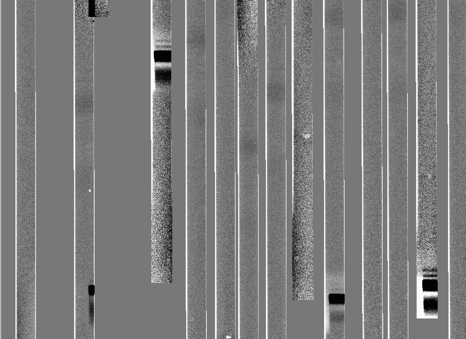
Now we are ready to biasflat ccd005:

biasflat -f ccd003_flat ccd005

The output will be a set of images files ccd005_f. Here's what the same section of a flattened spectrum frame looks like:

Top

Step 7: Processing the spectra

The next step is to subtract the sky using the routine subsky.

subsky -m ccd004_b -f ccd005_f

or

subsky -m ccd004_b -f ccd005_f -z mybadfile

which produces a set of image files ccd005_s, a section of which looks like this:

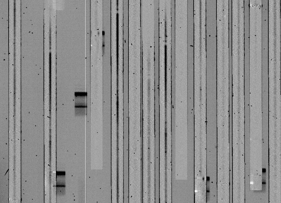
If the comparison arcs are well-matched to the object frames, the sky subtraction should usually be this clean, but it might not for several reasons:

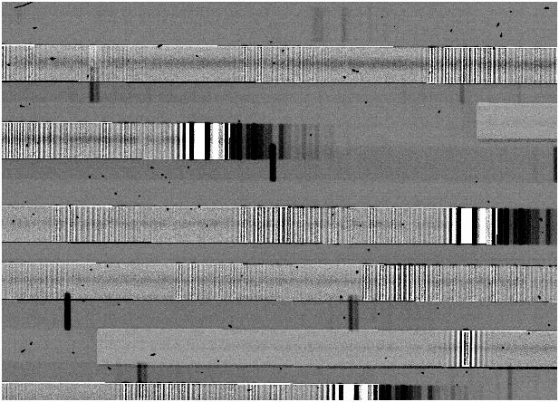
• If the spline fit parameters are not set properly, the spine fit can become unstable, creating ringing. The result will be an image which looks like this:
  
• For reducing IMACS exposures with short slits, a 1-d spline fit is usually more than adequate, and is much faster than the 2-d spline fit. However, if your slits are long, and particularly if the objects sit on a variable background, you may see a significant slope across the sky subtracted spectra. In that case, use a 2-d spline.
• Another time when 2-d splines are useful is when the spectral map does not perfectly describe the tilt of slits, resulting in residuals which look like this:
  

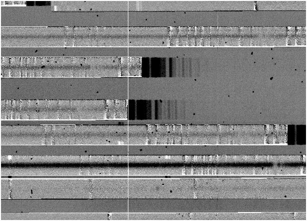
This seldom occurs with IMACS, but does seem to be more common with LDSS3. In this case, switching to a 2-d fit and selecting to fit the tilt should solve the problem.

Occasionally, the spline fit for a spectrum does not converge. In this case, you will get a message like this:

Problem fitting sky of slit 2, chip 6 0 (1)

and this spectrum will be set to zeroes.

We are now ready to extract the spectra using extract-spec. You have four choices:

1. Do a 2-d extraction on each object exposure, then use sumspec to combine the frames with cosmic-ray rejection.
2. Do step 1, then extract 1-d spectra from the combined image with 1dspec.
3. Do a 1-d extraction of each exposure, with cosmic-ray rejection, then combine these with sumspec.

If the spectra are reasonably strong, there is little to choose between methods 2 and 3. With very weak spectra, method 2 may sometimes be preferable. Alternatively, you may:

4. Using the spectrum mapping in the map file plus the sky subtracted spectral frames, design a custom extraction procedure. See Writing routines for COSMOS for more details on this.

We will illustrate method 2..

First, we extract each object exposure

extract-spec -m ccd004_b -f ccd005_s

extract-spec -m ccd006_b -f ccd007_s

If the search parameter has been set to a non-zero value, extract-spec will present various plots of spectrum shape and offset.

Now, having turned on cosmic-ray rejection in the sumspec parameter file, we do:

sumspec -o Mymask_2spec ccd005 ccd007

Note that we don't specify any spectrum type (like _2spec) for the input files, but must for the output file. Finally,

1dspec Mymask

Top

Constructing Bad Pixel Maps

A bad pixel map exists for each dewar, in the directory $COSMOS_HOME/sdata, with the name dewar.badpix. This file maps the location of known bad features on each chip. These files contain, the coordinates of bad pixel groups, one per line. The format is:

chip      xmin     xmax    ymin    ymax

Unless another bad pixel map is specified on the command line, Sflats and subsky use the standard files, however the user can construct and use his/her own bad pixel file, either from scratch, or using the standard files as a starting point.

In addition to bad pixels on the chips, it is often useful to block regions where unwanted spectral orders overlie the desired spectrum. This can be done by constructing a new bad pixel file for each observing setup, using the program badorders. badorders requires, as input, an observation definition file specific to each spectral order to be blocked. These files will differ from the standard observation definition file for the observing setup in the spectral order specified, and probably also in the dewar offset file, since there are usually small order-to-order differences offsets between the true positions of spectral features and those predicted by the optical model.

Constructing an appropriate dewar offset file for each order may take some work. Since the orders that one wants to block are those which lie on top of the desired order, align-mask may or may not be successful in determining a correct alignment because of the confused image. If it does not work well, it will be necessary to create one for the order by adjusting the dewar offset file created for the primary order, using adjust-offset.

Don't forget:

• if you create the new dewar offset file with align-mask: align-mask names the dewar offset file from the arc file, so you must take care to rename each dewoff file to specify the order to which is applies, and take care that the original primary order offset file doesn't get overwritten.
• if you create the new dewar offset file with adjust-offset: first rename the primary order offset file to something specific to each order before running adjust-offset.

Top

Reducing Nod&Shuffle data

Although the COSMOS routines handle most aspects of Nod&Shuffle data automatically, there are some aspects of N&S data reduction that must be noted:

• Comparison arcs should not be shuffled. adjust-map does not use the shuffled images, and their proximity to the primary comparison lines may cause problems for the fit.
• Spectral flats may either be shuffled or not shuffled. If not shuffled, the shuffled parameter in Sflats should be set to the shuffle distance of the data, so that a shuffled flat field file is produced.
• N&S spectra should be processed through subsky, even though no sky subtraction is done to the data, so that subsky can produce the data plane with pixel errors that are needed in the later reductions.
• extract-spec extracts the shuffled regions along with the primary spectra. If the parameter sub_ns is set to "yes", the shuffled regions are subtracted from the primary spectra to subtract sky. This should be done if spectra are later to be combined, with cosmic ray rejection, using sumspec.
• viewspectra can handle 2-dimensional N&S data produced by extract-spec that either has or has not had the shuffled region subtracted. If the region has not been subtracted, the shuffle parameter should be set to "yes", and the shuffled region is subtracted before display and analysis. The 1-d spectral plots show the spectrum after subtraction of the (negative) nodded spectrum.

Top

Reducing LDSS3 data

Reducing LDSS3 data is very similar to IMACS with a few minor changes:

• In defineobs select LDSS3.
• All data frames need to be stitched together before the alignment using the COSMOS routine stitch. The IRAF routine lstitch will not work with COSMOS.
• The biasflat parameter DEWAR needs to be changed to "LDSS3", since stitch takes care of all the gains and biases.
• In subsky and Sflats, you need to change the NOISE and GAIN values, which can be found here.
• For newer LDSS3-C data (data taken after March 2014), make sure you set DEWAR to "LDSS3C-2". All of the other programs are run the same way as you would on older LDSS3 data.
• Note that LDSS3-C data taken in Normal mode is in Normal orientation (spectra dispersed vertically), so be sure to use a dewoff file ending in "_N.dewoff". Dewoff files are located in $COSMOS_HOME/sdata/dewoff

Top

Reducing Longslit data

Longslit data can be taken for IMACS or LDSS3. COSMOS can correct for line-curvature to produce rectified longslit data.

• The initial dewoff alignment must be done with adjust-mask instead of align-mask. Refer to Creating and Modifying Dewoff Files documentation for specifics of modifying dewoff files.
• Turn on the fit_curv parameter in the adjust-map parameter file in order to enable fitting for the curvature.
• If there is a lot of scatter in the curvature plot, remove blended or confused lines from the line list or decrease the line rejection threshold.
• By running subsky on a lamp frame, using the map from adjust-map, you can inspect how well the line tilt and curvature is being fit. Badly fit lines will have P Cygni profiles which vary along the slit.

Top

Pipelining the reductions

Once all this becomes routine, i.e. you know how all the programs behave and how your data behaves, you can put everything from the map-spectra procedure onward into a script, using process-spec. Note the restrictions listed in the web page before running.

process-spec

Spectrum set:           Mymask_night1

Associated obsdef file: Mymask

Bad pixel file:         Mybadfile

Science frame #         005

    Bias frame:         bias

    Comparison arcs:    004 006

    Flat frames:        005

Science frame #         007

    Bias frame:         bias

    Comparison arcs:    006 008

    Flat frames:        009 010 011

Science frame #

Spectrum reduction makefile Mymask_night1.make created

The script Mymask_night1.make can be executed using the standard UNIX command make.

make -f Mymask_night1.make

Top

Next: Creating and Modifying Dewoff Files

Back to Table of Contents