A COSMOS Cookbook

The following describes some procedures for handling data reduction tasks. For detailed information on each of the programs the reader should refer to the web pages for that program.

Reducing multislit spectra

Let's assume that you have a mask named Mymask, and you have obtained the following set of observations with IMACS using the short camera in Nod&Shuffle orientation, and the 200 line grism

Frame	Exposure
ccd001	bias
ccd002	direct mask image
ccd003	spectroscopic flat
ccd004	comparison arc
ccd005	spectrum
ccd006	comparison arc
ccd007	spectrum
ccd008	comparison arc
ccd009	spectroscopic flat

Step 1: setting up the environment

COSMOS assumes that all the data files except the FITS image files are in the current working directory, but that the FITS files are in the directory pointed to by the environment variable COSMOS_IMAGE_DIR. Everybody has their own preferences for arranging files; one convenient way is to have all the data files for an observing run in a directory dir, with subdirectories n1,n2, ... for each night's FITS files. You should cd to the directory in which you will keep and use the non-image files, then used setcosdir to specify the image directory. With the above suggested directory structure, to work with image files in the n1 subdirectory, you could either define COSMOS_IMAGE_DIR as ".",- i.e. the current directory- and refer to image files as n1/filename, or define COSMOS_IMAGE_DIR as "/home/joe-users/...../dir/n1", and refer to image files as filename.

Step 2: setting up observation definition files

We need to set up an obsdef file for the spectroscopic observations. It also doesn't hurt to first check the direct image of the mask, just to ensure that there are no major problems. For this we need a direct image obsdef file as well.

we invoke defineobs and insert the following data for the direct image:

Instrument:	IMACS
Mask:	Mymask
Dewar Offset File	SCdirect_NS
Camera:	SHORT f/2
Mode:	DIRECT
Observation Definition File	Mymask-direct

and for the spectroscopic observations, the following:

Instrument:	IMACS
Mask:	Mymask
Dewar Offset File	SC200g_NS
Camera:	SHORT f/2
Mode:	SPECTROSCOPIC
Grism:	200l
Observation Definition File	Mymask

Note that we have specified the instrument as "IMACS". This is correct for data taken before August 01, 2005, when chip 6 was replaced in the SITE dewar. After August 01, the instrument should be identified as "IMACS2".

Because we have not yet used align-mask on any images, we have used the default dewar offset files, which are located in $COSMOS_HOME/examples/dewoff. When finished, we now have two obsdef files: Mymask-direct.obsdef, and Mymask.obsdef.

Step 3: Aligning masks

It's usually not even necessary to look at the direct mask images, but let's do that anyway just to make sure everything is OK (useful to do, for example, at the beginning of a run). First, we set the parameters in align-mask

editpar align-mask

type q to end

SEARCHBOX                   10       half width of search range
MAGFACTOR                  100       magnification factor for offset vectors
LAMFILE                HNA.dat       line list file
NAVER                        1       number of neighboring points to average is plot

Change parameter:

A searchbox of 10 is usually sufficient; if most apertures cannot be found, increase it to 20. The lamfile is only needed for the spectroscopic image alignment.

Now, run align-mask to check and correct the alignment.

align-mask -o Mymask-direct -f ccd002

After the first iteration, assuming that it is successful, rerun defineobs and insert ccd002 as the name of the dewar offset file. The second iteration should show quite good agreement.

Assuming that this worked well, we are ready to align the spectroscopic images.

If it didn't work:

If it did not work well, something may be very wrong. In that case we should generate a list of predicted positions using apertures and overlay it in IRAF with the mosaiced image.

apertures -o Mymask-direct -b 1 (assuming you used 1x1 binning)

In IRAF:

display8 ccd001 1 z1=0 z2=whatever
tvmark 1 Mymask.xy

A comparison of predicted and observed apertures positions should allow you to understand the problem.

Assuming it did work:

Now we need to align the spectroscopic mask. We only do this once, using one of the exposures, for a set of spectroscopic exposures that we want to reduce as a group and combine (even though flexure may result in slight shifts from one exposure to the next.) The reason for this will be explained later. We need to specify a line list file in the align-mask parameter file. This list should consist of a small number of clean, well-isolated comparison lines. In this example, we have called it HNA.dat, and specified that in the align-mask parameter file. Having done so:

align-mask -o Mymask -f ccd006

Again, change the name of the dewar offset file in Mymask.obsdef to ccd006 after the first iteration. The second iteration should look pretty good, like this:

align mask

The typical residual is about a pixel, and is dominated, as is obvious, by systematic errors. These are due to imperfectly-mapped distortions in the IMACS optics. These small errors will be removed later when we construct and adjust the spectral map.

Step 4: Constructing the spectral map

The spectral map is a file which contains the information necessary to transform from CCD coordinates to the space of wavelength vs slit position into which we want to transform our data. The information necessary to construct a first, approximate map (which should be good to a few pixels) is all contained in the observation defintion file. The map is constructed using the program map-spectra. So:

map-spectra Mymask

We will do this only once for each set of data which we wish to combine. Because this map is approximate, we use the comparison arc exposures to adjust it in the most suitable way for each sicence spectral exposure, using adjust-map. We can use a single arc exposure, or interpolate between two. adjust-map works best with bias-subtracted frames; In our example, each science exposure is bracketed by two arc exposures, so we can do:

biasflat ccd004 ccd006

      

then

adjust-map
-m Mymask -f ccd004_b ccd006_b

which will produce a new map file ccd004-6_b.map to use with the science exposure ccd005, and so forth. To repeat what was stated earlier, if we wish to later combine ccd005, and ccd007, with cosmic ray rejection, we should start with the same basic map file, Mymask.map, created from one observation definition file, Mymask.obsdef.

Care must be taken to pick a good list of comparison lines. Make sure that all chosen lines are clean and well-isolated, lines near to stronger lines are particularly to be avoided. Particularly when using a new line list, or a new instrumental setup, it is wise to first run adjust-map in debugging mode, so that you can see how the dispersion fits are working: you may find that one line is consistently not behaving well, or that the order of the adjustment is too high or low. It's also not a bad idea to check the map file output created by adjust-map, by using spectral-map to create a list of expected spectral line positions, then overlaying them on the image of the arc frame.

spectral-map -m ccd004-6_b -l linelist.dat -b 1

where linelist.dat is a file containing a comparison arc line list. Then, in IRAF

display8 ccd004 1 z1=0 z1=whatever
tvmark 1 ccd004-6_b.xy

The marked positions should align virtually perfectly with the slit centers (to within the pixilization). If they're still off, try repeating adjust-map:

adjust-map -m ccd004-6_b -f ccd004 ccd006

That should do it quite well. If it doesn't, its probably due to a bad line fit. adjust-map produces a file called adjust-map.dat, which contains details of the line offset determinations. See the web page for adjust-map for details. Look at the values of delta(x) for the spectrum which is giving problems. There will probably be one discrepant value. Chances are that inspection will show that this line is being influenced by a neighboring line; if so, delete it from the line list and repeat the fit.

Step 5: Preparing the frames

We now need to do bias subtraction and flat-fielding of the science exposures, using biasflat. Since we will use the same bias frame for all science exposures, we can identify it in the biasflat parameter file, but we will need to specify different flat-field frames on the command line for each science exposure. We create spectroscopic flat fields for the science exposures using Sflats, in our case

Sflats -m ccd004-6_b -f ccd003

will create a set of image files ccd003_flat which we will use with ccd005. Sflats normally uses the standard bad pixel file for each dewar, to mask out bad regions of the chips. If you have created your own custom bad pixel file for a mask, for example to mask out zero order grism images, you would say

Sflats -m ccd004-6_b -f ccd003 -z mybadfile

Here's what a section of one of these frames looks like:

sflat image

Now we are ready to biasflat ccd005:

biasflat -f ccd003_flat ccd005

The output will be a set of images files ccd005_f. Here's what the same section of a flattened spectrum frame looks like:

Step 6: Processing the spectra

The next step is to subtract sky using the routine subsky.

subsky -m ccd004-6_b -f ccd005_f

or

subsky -m ccd004-6_b -f ccd005_f -z mybadfile

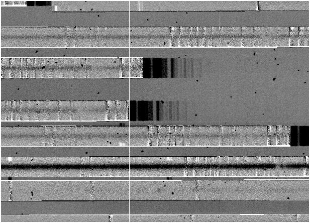
which produces a set of image files ccd005_s, a section of which looks like this:

sky subtracted frame

If the comparison arcs are well-matched to the object frames, the sky subtraction should usually be this clean, but it might not for several reasons:

If the spline fit parameters are not set properly, the spine fit can become unstable, creating ringing. The result will be an image which looks like this:

For reducing IMMACS exposures with short slits, a 1-d spline fit is usually more than adequate, and is much faster than the 2-d spline fit. However, if your slits are long, and particularly if the objects sit on a variable background, you may see a significant slope across the sky subtracted spectra. In that case, use a 2-d spline.
Another time when 2-d splines are useful is when the spectral map does not perfectly describe the tilt of slits, resulting in residuals which look like this:

This seldom occurs with IMACS, but does seem to be more common with LDSS3. In this case, switching to a 2-d fit should solve the problem.

Occaisionally, the spline fit for a spectrum does not converge. In this case, you will get a message like this:

Problem fiting sky of slit 2, chip 6 0 (1)

and this spectrum will be set to zeroes.

We are now ready to extract the spectra You have three choices:

Do a 2-d extraction on each object exposure, using extract-2dspec, then use sumspec to combine the frames with cosmic-ray rejection.
Do a 1-d or 2-d combining+extraction+CR rejection using extract
Using the spectrum mapping in the map file plus the sky subtracted spectral frames, design a custom extraction procedure. See Rolling your own for more details on this.

Method 1 is the most robust at the present time, so we'll do that.

First, we extract each object exposure

extract-2dspec -m ccd004-6_b -f ccd005_s
extract-2dspec -m ccd006-8_b -f ccd007_s

If the search parameter has been set to a non-zero value, extract-2dspec will present various plots of spectrum shape and offset.

Now, having turned on cosmic-ray rejection in the sumspec parameter file, we do:

sumspec -o Mymask_2spec ccd005 ccd007

Note that we don't specify any spectrum type (like _2spec) for the input files, but must for the output file.

Reducing Nod&Shuffle data

Although the COSMOS routines handle most aspects of nod&shuffle data automatically, there are some aspects of N&S data reduction that must be noted:

Comparison arcs should not be shuffled. adjust-map does not use the shuffled images, and their proximity to the primary comparison lines may cause problems for the fit.
Spectral flats may either be shuffled or not shuffled. If not shuffled, the shuffled parameter in sflats should be set to the shuffle distance of the data, so that a shuffled flat field file is produced.
N&S spectra should be processed through subsky, even though no sky subtraction is done to the data, so that subsky can produce the data plane with pixel errors that are needed in the later reductions.
extract-2dspec extracts the shuffled regions along with the primary spectra. If the parameter sub_ns is set to "yes", the shuffled regions are subtracted from the primary spectra to subtract sky. This should be done if spectra are later to be combined, with cosmic ray rejection, using sumspec.
viewspectra can handle 2-dimensional N&S data produced by extract-2dspec that either has or has not had the shuffled region subtracted. If the region has not been subtracted, the shuffle parameter should be set to "yes", and the shuffled region is subtracted before display and analysis. The 1-d spectral plots show the spectrum after subraction of the (negative) nodded spectrum.

Pipelining it

Once all this becomes routine, i.e. you know how all the programs behave and how your data behaves, you can put everything from the map-spectra procedure onward into a script, using process-2spec. Note the restrictions listed in the web page before running.

process-2spec

Spectrum set:	Mymask_night1
Associated obsdef file:	Mymask
Bad pixel file:	Mybadfile

Science frame #	005
Bias frame:	bias
Comparison arcs:	004 006
Flat frames:	005

Science frame #	007
Bias frame:	bias
Comparison arcs:	006 008
Flat frames:	009 010 011

Science frame #

Spectrum reduction makefile Mymask_night1.make created

The script Mymask_night1.make can be executed using the standard unix command make.

make
-f Mymask_night1.make