Why does GALFIT require image data values to have units of [counts], as opposed to count rate [counts/sec], [MJy/sr], or other units, for generating sigma images?
Strictly speaking it doesn't, but it's a really good idea for avoiding subtle and easily preventable mistakes. What GALFIT really needs is for the units of pixel ADU × GAIN to be [electron], the basic counting unit, if you want GALFIT to generate the sigma image for you. And there are other combinations where that is true that would work (see below). First, a clarification (hopefully) on the usage of the terms counts and ADU: An ADU (Analog-to-Digital Unit) is a scale factor that relates the number of elections in a pixel with a pixel value. There are many reasons why it may not be desirable for 1 ADU to equal 1 electron. Regardless of the reason, it is pretty fundamental for data analysis to want to know how many electrons went into producing a pixel value, and GAIN is the keyword that usually comes to mind. As far as units are concerned, an ADU is rather like a metaphysical unit because it has whatever unit a pixel value has, and the units of a pixel can be a lot of things. But in common usage ADU is used interchangeably with "counts." When a pixel value has flux units, it is more common to explicitly say "ADU per second" or "counts per second," even though an ADU can equally well be defined as a flux unit. This FAQ uses ADU (≡ count) to explicitly differentiate from ADU/sec (≡ count/sec).
Confusion sometimes creeps in when, during data processing, the units for GAIN don't get propagated along even as the image pixels change units from, say [counts], into [counts/sec], [MJy/sr], etc.. When that happens, the GAIN parameter lives on as a meaningless thing in the header. As mentioned earlier, knowing how to go from image ADU into [electrons] is fundamental to data analysis, for which GAIN is the most obvious go-to keyword (even if there is another, having GAIN be present alongside that other is just as confusing). GALFIT either needs to have, or needs to create, a σ-image to fit an image, as explained in more detail here, and mixing units can be costly.
So the notion that GALFIT likes the ADUs to have units of [counts], and not [counts/sec], refers to when the units for GAIN remains unchanged from its initial definition, after data processing, which happens more often than not. So, if you want GALFIT to create the σ-image, it is important to always first figure out what are the units for GAIN. However, the important points that you should take away when working with GALFIT are these:
- If you don't want GALFIT to generate the σ-image and have an external way to do so, you can ignore everything in this section.
- Since GALFIT requires ADU × GAIN to have units of [electrons], there is more than one combination of units that would work because the units for ADU can in principle be anything. One example is for the data to have units of [counts sec-1] and the GAIN to have units of [electrons / (counts sec-1)]. Likewise, if the data units are in [MJy sr-1] and the GAIN has units of [electrons / (MJy sr-1)], then that will also work. Be mindful that if GAIN is altered from the original instrumental definition, you may or may not need to set NCOMBINE to 1, depending on whether NCOMBINE is already factored into GAIN.
- If the GAIN header keyword retains its original, instrumental definition, but your pixels are in some other units, then you either need to convert the image back into [counts], or else you have to change the GAIN header value so that the units [ADU] × [GAIN] = [electrons]. Due to the importance of measuring good sky value, it is often better to work with images that are in the original instrumental [counts] rather than other units, e.g. [counts/sec].
What Happens If You Provide GALFIT an Image with the Wrong Units for Generating the Sigma Image?
For GALFIT to produce reliable σ images, the data ought to have proper units for GALFIT to convert data values into electrons via the GAIN parameter. Nevertheless, this notion is very abstract, and it is easy to neglect the importance especially when visual inspections show that the residuals look good. So just how much does it matter?
Below are two sets of simulation, both provided to me by Takahiro Morishita (Tohoku University of Japan). The first set (Figures 1, 2, and 3) shows what happens when the image pixels have units of [counts/sec] whereas the GAIN is in [electrons/ADU], with ADU being in [counts] rather than [counts/sec]. The last figure shows the same analysis he performed on simulations where the image pixels have units of [counts]. His simulations, being such a beautiful example of this issue, I asked permission to share them with the public.
Figure 1 shows simulations of idealized Sérsic n < 2.5 and n > 2.5 galaxies, based on fitting images where the data numbers have units of [counts/sec] but the image GAIN has units of [electrons/count], allowing GALFIT to generate the σ-image for the fit. The galaxies were placed into blank fields, without neighbors, with idealized Poisson noise. The top panel shows the magnitude offsets between the output and input magnitudes, where the output magnitudes get systematically fainter compared to the input. The upward trend is quite noticeable and significant even at fairly bright magnitudes. The output sizes in the middle panels show a large systematic trend toward smaller output sizes. And the output Sérsic index values are systematically underestimated.
FIT RESULTS WHEN THE UNITS of [ADU] × [GAIN] ≠ [electrons];
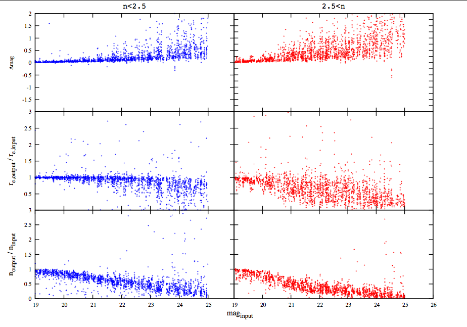
Figure 1: Output fit parameter deviations as a function of input magnitude for single component, idealized galaxies with Sérsic profiles. The galaxies are isolated and have idealized noise. Left: Sérsic indices n < 2.5. Right: Sérsic index values n > 2.5. Top: Differences between output and input magnitude. Middle: Ratio of output and input sizes. Bottom: Ratio of output and input Sérsic index values. Provided by Takahiro Morishita.
At this stage in the analysis, it is natural to think that these behaviors are to be expected for several plausible (but wrong) reasons: a notion commonly expressed is that as objects get fainter, it gets harder for an algorithm to "see" the faint wings of galaxies, therefore it is natural to measure smaller sizes for fainter objects. Another common belief is that the large scatter and systematics reflect the fact that the parameters are highly correlated, which become more and more difficult to disentangle in the presence of noise. Then there is the notion that parameter degeneracy is a serious issue when using Levenberg-Marquardt techniques. The above plot may seem to give credence to such notions, which may lead one to accept that some level of systematics are unavoidable limitations of the analysis technique.
If one were to accept the above ideas as being true, then it may lead one to take the next logical step, which is to try and remove the systematic biases by fitting a function to the simulation data, and subtracting out the median trend from the individual data points. The result should, in principle, have no bias in the median. Doing so to the magnitude and size parameters produces the following two Figures:
RESULTS AFTER SUBTRACTING OUT THE MEDIAN TREND IN MAGNITUDE FROM FIGURE 1
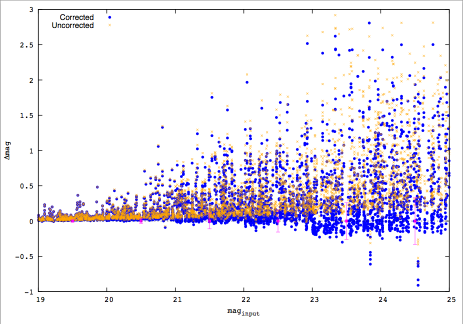
Figure 2: An attempt at correcting the systematics in magnitudes by subtracting the best fitting median trend in Figure 1. Note the large scatter remains, and the scatter is nevertheless non-symmetric even when the median is now effectively zero. Provided by Takahiro Morishita.
RESULTS AFTER SUBTRACTING OUT THE MEDIAN TREND IN SIZE FROM FIGURE 1
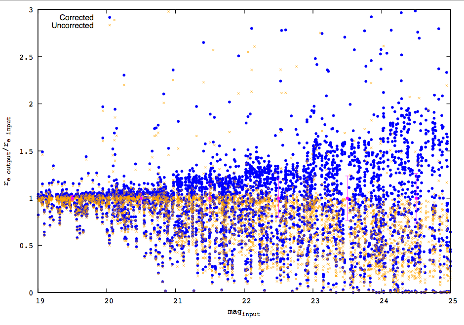
Figure 3: An attempt at correcting the systematics in size by subtracting the best fitting median trend in Figure 1. Note the large scatter remains, and the scatter is nevertheless non-symmetric even when the median is now effectively zero. Provided by Takahiro Morishita.
Notice that despite removing the median trends, the scatter and the trends remain quite dramatic. Without any other basis for comparison or external sanity checks, it may seem this is the best one can do. The scatter and the trends are taken to indicate the intrinsic limitations of this analysis approach. In some studies of recent past, such an approach has been used to critique both the technique, and science results drawn from it for not having made such "bias corrections."
In contrast to the above approach, Takahiro Morishita produced a plot showing test results when the same simulations as above are run using data with the correct unit of [counts], with GAIN in [electrons/count], rather than in flux rate units above:
FIT RESULTS WHEN THE IMAGE HAS CORRECT UNITS WHERE [ADU] × [GAIN] = [electrons]
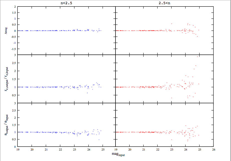
Figure 4: The same simulation set as Figure 1, except where the pixel units pair up correctly with GAIN, which GALFIT expects for producing a σ-image. Compare with Figure 1 to see the dramatic differences in the scatter and systematic trends between the two figures. The two plots are shown at the same scale. Provided by Takahiro Morishita.
Clearly, the intrinsic scatter and the systematics are much smaller when the units are correct for generating the σ-images, compared with Figure 1.
In summary, getting the units right is very important if one wants GALFIT to generate accurate σ-images. Working with images in [counts/sec] when the GAIN is in [electrons/count] may seem on the surface to be perfectly fine. However, when GALFIT is asked to generate a σ-image based on images with the wrong units, in all likelihood the measurement accuracy will not be good. Even if one can "correct" for biases, such an approach may not be reliable. In fact because the σ-images would be wrong, the noise properties in simulations would likely be different from the noise properties of actual data. If so, the fits may be biased in different ways when applied to real data, even after "bias corrections." Perfectly idealized simulations ought not show systematics, to any significant extent, if the simulations are produced correctly. If one cannot accurately recover idealized simulations parameters, whether for galaxies in isolation or placed into real images, it is a warning sign that the data units (or the gain) may not be correct for GALFIT to generate a reliable σ-image.
 )
)